Дипломная (вкр): Predicting completion of cash acquisitions using option implied risk-neutral probabilities

 was restricted to 0 and =1-. To eliminate the effect of potential information leakages or market fluctuations the pre-announcement price was taken as a five-day average 2 weeks before the announcement, while fallback price - five-day average 2 weeks after the resolution. both probability forecasting approaches daily predictions were gathered into weekly by taking the 5-day average and then probit regressions of the deal's outcome (was viewed as a binary event: 1 in case of success and 0 in case of failure) on both estimates jointly and separately were fitted for each week. Predictive power of risk-neutral and naïve probabilities was compared on the basis of pseudo- and significance of coefficients. research is finalized with a brief evaluation of merger arbitrage and its dependents on the option-implied probability of success. After the M&A announcement stock of the target company generally trades at a price below the one offered by acquiring company. The difference between target’s stock price and the offer price is commonly known as arbitrage spread. Merger arbitrage, or risk arbitrage, is an investment strategy that makes an attempt to profit from this spread. For cash offers the strategy is to simply buy the target’s stock and hold it until the deal’s resolution, expecting to sell it at the offer price if the offer is successful. The key feature to point out is that risk of this strategy is not linear. In case of the offer’s success investor captures the arbitrage spread, but if the deal fails he incurs a loss that is usually larger than profit that would have been obtained if the deal succeeded. Therefore, inside on the probability of the deal’s success could potentially improve the excess returns from merger arbitrage strategies. evaluate the hypothesis whether obtained risk-neutral probability forecasts have any implications regarding potential merger arbitrage profits on the stock market 4 different portfolios (featuring different share of stocks depending on their respective risk-neutral probability forecasts) were constructed using the chosen sample and their returns were compared to each other and to the chosen benchmark (returns on Hedge Fund Merger Arbitrage index) that was used in excess returns estimation.

Empirical results. Risk-neutral probability forecasts and their predictive power

For the sample of 164 deals probability of the tender offer success was calculated using equation 10 for each trading day during the chosen period of 3 weeks after the announcement and 3 weeks before the resolution (denoted as week -3, week -2 and week-1). 24 of the deals didn’t have quoted option prices through out the whole 6-week period and for 11 deals no combination of bid and ask could guarantee convexity and, thus, they were excluded from the sample. For the remaining 129 deals, out of which 100 succeeded and 29 failed weekly forecasts were calculated by taking five-day average.display the option-implied probability forecasts and gain additional inside on their predictive power each weekly forecast was assigned to one of 6 subintervals: [0.0; 0.1), [0.1; 0.2), [0.2; 0.4), [0.4; 0.6), [0.6; 0.8) and [0.8; 1). These intervals will further be referred as 0.05, 0.15, …, 0.5, 0.7 and 0.9 probability categories. Taking Statistical limitations into account, finer partition is undesirable, as it would imply weaker statistical tests. forecast distribution is shown in Figure 1. It is worth noting that successful offers make up approximately 78% of the sample. Assuming that sample is representative, we can denote this proportion as “prior” probability of success for the typical target. Thus, unsurprisingly largest proportion of forecasts fall into 0,7 category during week 1 and 2 after the announcement. However, for successful offers the proportion of forecasts in top 0,9 category increase significantly over 6 weeks (from 28% in week 1 to 43% in week -1). As expected, the exact opposite can be observed for unsuccessful deals: the share of forecasts for unsuccessful takeovers that fall into lowest probability category (0,05) increase from 20,1% in week 1 to 41,4% in week -1. Another important trend to point out is that proportion of “successes” in top 2 categories increase from 96,9% in week 1 to 100% in week -3 and onwards. All of the above may suggest that our forecast captures true probability quite well and its predictive power tend to increase when closer to resolution date.

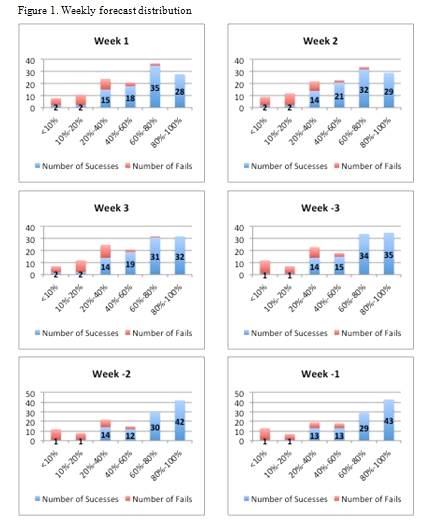
Table 4. Brier score

4 reports weekly Brier scores featuring base rate, calibration and resolution components. Brier score monotonically decreases and the main conclusion that can be drawn is that market’s forecasting ability significantly increases as resolution date becomes closer. The interpretation of the Brier score, as mentioned by Samuelson, Rosenthal (1986), can be conveniently described as follows: a Brier score of  in terms of forecasting performance is equivalent to a probability forecast of  that is right  of the time. For example, week’s 1 Brier score of 0,165 is equivalent to a 79,2% forecast that is right 79,2% of the times. Week -3 scores an 83,9% correct forecast equivalent while week -1 is equivalent to 85,2% correct forecast.all of the weeks Brier score is substantially lower than the base rate component. If the market had used the base rate frequency of success to access all offers at 78% success probability, it would have been right only 78% of the time. By conducting a chi-squared test on a sample variance we test the hypothesis that the difference between obtained Brier score and base rate is statistically insignificant. Table 3 provides the resulting p-values, rejecting H0 of no difference at 5% significance level for all weeks and at 1% significance level for all weeks except for week 1.insight can be gathered from analysis of calibration and resolution components of Brier score, as they are the source of forecasts’ performance weekly improvement. Calibration and resolution of forecasts both improve over time, with calibration component falling while resolution component rising, on average. Brier score’s improvement, on average, is mainly driven by resolution component’s increase. Resolution component is also the source of a significant drop of the Brier score in week -3 compared to week 3. However, we observe jumps of calibration and resolution components in a 3-week post-announcement period. For week 2 calibration slightly worsens compared to week 1 and a trade off occurs between resolution and calibration that was mentioned in the methodology section. For week 3 calibration falls to the initial week 1 level, while resolution stays unchanged compared to week 2. On average, however, these effects balance in such a way that Brier score monotonically improves.well are the obtained probability forecasts calibrated? To answer this question we will analyse a break down of observed success frequencies by probability category and week presented in Table 5. Reviewing these frequencies yields a conclusion that they are highly correlated with our predicted probability estimates, but considerably greater in most cases. Under null hypothesis that  is the true success probability for tender offers falling into the j-the category number of successes follows a binominal distribution with mean  and variance . We then test this hypothesis using standard t-test against the two-sided alternative and an Unconditional Coverage test with likelihood ratio given by: 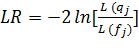. Table 5 reports p-values for both tests. Note that for category 0,7 and 0,9 success rate is 1 in most of the cases and, thus, Unconditional Coverage test is not applicable. In general, p-values are very low, rejecting the hypothesis that that  is the true probability of success for the offer falling into the respective probability category. At 5% significance level only 14 cells out of 36 for t-test and 12 out of 27 for Unconditional Coverage test cannot reject H0. Note that in our case tests provide slightly different results, rejecting H0 for different sells. Rejections are mainly concentrated in 0,3, 0,5 and 0,7 probability categories and suggest that market severely underestimates the success probability for tender offers falling into these categories. However, small sample size limits tests’ power and, therefore, we cannot treat the above-mentioned results as a definite sign of market inefficiency. Generally, we observe that risk-neutral probability forecasts tend to underestimate the true probability of success, as for nearly all entries in the table observed frequencies are higher than the option-implied probability estimates. Despite their significant predictive power, option-implied probability forecasts appear to be poorly calibrated.

5. Calibration tests

verify this proposition let’s consider the output of weekly probit regressions of the deal outcome on the risk-neutral probability forecasts. Table 6 reports results of these regressions, including pseudo , coefficients and p-value of the coefficient before the probability estimate. We observe that forecasting power of the probability estimates increase significantly closer to resolution, once more, supporting the interpretation of Brier score improvement. Pseudo improves from 32,9% in the first week after the announcement to 55,1% in the week prior to resolution. However, by looking at coefficients in probit regression without intercept we can denote that they are significantly higher than one (ranging from 2,19 to 2,43 for all weeks). This finding suggest that option-implied probability forecasts, indeed, under predict the probability of a cash takeover success, supporting the insight gathered from calibration component analysis of the Brier score. substantial gap between risk-neutral probability estimates and ex post realized frequency suggests that options on target companies could be undervalued and indicates a potential to earn excess returns once an appropriate investment strategy is chosen.

6. Probit regression

Comparative analysis of option-implied and stock-implied forecasts

We continue the analysis of forecasts’ performance by comparing their predictive power with that of “naïve” probabilities derived from stock prices. Recall that “naïve” probabilities are defined, as in Samuelson and Rosenthal (1986) and given by:

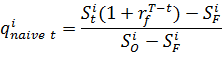
-price of the stock at time t, -fallback price, -offer price per share, (T-t)-time to deal resolution, - risk-free rate for the appropriate perioda regression for a fallback price of failed deals on pre-announcement price and offer price yields the following result (standard deviation of the coefficient in parenthesis), suggesting that pre-announcement price and offer bid predict fallback price quite well:

   (0,07)

the obtained fallback price estimates into the probability formula we obtain the weekly “naïve” probability forecasts for our sample of 129 deals and then compare them with option-implied probability estimates. For many of the deals stock-implied probabilities were outside the desired [0;1] range and, thus, those deals had to be excluded from the comparative analysis. Table 7 summarizes the results (pseudo-  and p-values for coefficients) of cross-sectional probit regressions for each week and for the 6-week average. results of the comparisons are mixed. For the first 3 weeks after announcement and for the week that is 3 weeks before resolution risk-neutral forecasts generate, on average, larger pseudo , suggesting to have higher predictive power than “naïve” probabilities. However, the situation is reversed, as resolution date approaches. 2 weeks before resolution “naïve” probability estimates experience a significant jump of their predictive power and start to outperform risk-neutral probability forecasts (pseudo  of 50,3% compared to 44,4% for week -2 and 63,0% compared to 47,6% for week -1 respectively). For the average of the 6-week period risk-neutral forecasts, indeed, outperform “naïve” ones in terms of predictive quality (pseudo  of 41,8% compared to 36,8%).regression of deal outcome on both probability estimates suggest that predictive power of the model is significantly higher when both forecasts are used in combination. Both estimates tend to be significant, with the exception for week -3 and week -1 for which the hypothesis of no significance is rejected at 1% level for “naïve” and option-implied forecasts respectively. All in all, no straightforward answer on whether option-implied probabilities outperform “naïve” ones can be given. For the period right after the deal announcement option market tends to react more wisely, implying better predictive power of risk-neutral probabilities. Closer to resolution, however, stock market revises its expectations and stock price movements become more informative. But option-implied probabilities still add significant value to forecasting deal outcome, especially when used in combination with stock-implied probabilities.

3. Probit regression output

Deal examples

Let’s now take a closer look at some of the deals from the sample. We first consider the bid by ConAgra to acquire Ralcorp that ultimately failed. This deal also provides an example of divergence between option-implied and stock-implied probability estimates and how it changed over time. The deal was announced on 29^th of April 2011 and the stock market reacted positively, indicating 75,5% success probability for the first week after the announcement. Ralcorp shares traded at and above $86 offer bid. However, this finding contradicted the unsupportive reception of the offer by the Ralcorp’s board. In the article published by the New York Times on 4^th of May it was outlined that Ralcorp commented that the offer “is not in the best interest of shareholders” and adopted a shareholder rights plan. The option market, on the contrast, showed little reaction to the announcement and risk-neutral probability of success was estimated to be 25,2%. Offer was withdrawn on 19^th of September. By that time bid price was raised to $94 dollars per share. Option-implied success probability dropped to 17,2% two weeks before the withdrawal and then to 2,8% one week before the withdrawal. Stock market still over predicted the success probability, estimating it to be 51,1% two weeks before the resolution. However, during one week before the withdrawal the gap between option-implied and stock-implied probability estimates shrank with stock market indicating probability of success to be 12,4%. 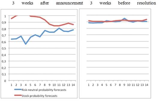Daily forecasted success probabilities for post-announcement and pre-resolution periods are shown in Figure 2.acquisition of Ariba, provider of cloud-based collaborative commerce applications, by SAP AG in 2012 is the example of a successful deal for which “naïve” probability estimates outperformed the risk-neutral ones for the period of 3 weeks after the announcement. On 22^th of May 2012 SAP AG, the largest maker of enterprise-applications software, announced to acquire Ariba Inc. for the price of $45 per share. This offer corresponded to 15% premium compared to average price of Ariba’s 2 weeks before the announcement. Market reacted with a price increase to $45 and the stock continued to trade approximately at the offer price for the following 3 weeks. The probability of success estimated from stock prices was 99,6%, 92,1% and 86,4% for weeks 1,2 and 3 respectively. Option market, on the contrary, didn’t react as sharply and estimated the success probability only at 63,8%, 72,8% and 77,6% for the above mentioned time periods. However, option market predictions improved significantly and converged to those of the stock market closer to resolution. One week before the resolution risk-neutral probability of success equalled to 90,5% while “naïve” method forecasted 92,0%. Figure 3 represents daily probability forecasts for both methods. Another important thing to notice is that we detect higher volatility for risk-neutral forecasts.2. Post-announcement and pre-resolution option-implied and stock-implied probabilities for Ralcorp.

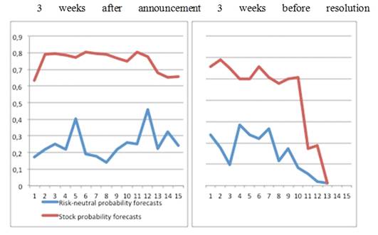
Figure 3. Post-announcement and pre-resolution option-implied and stock-implied probabilities for Ariba.

arbitrage and excess returns

’s now briefly consider practical application of the obtained risk-neutral probabilities to investment decisions and merger arbitrage. Recall that merger arbitrage (for cash deals) is a strategy associated with buying target company’s stock as soon as possible after the announcement and selling it at the resolution date. We define the excess return on a portfolio of stocks  as the difference between its return and the return on Hedge Fund Merger Arbitrage index provided by HFR database. This index aggregates the performance of merger arbitrage strategies of the whole hedge fund industry and is assumed to be a benchmark that carries the comparable level of risk. Table 4 summarizes information of excess returns associated with different portfolios. Based on the chosen sample equally weighted portfolio that is comprised of stocks that exhibited option-implied probability of success above 0,6 during first week after announcement generated the return of 4,2%, compared to 0,4% return of HFRX Merger Arbitrage index (Portfolio 4). If the investor didn’t bother with analysing success probability and simply invested equal shares in all target companies after the deal’s announcement the return would have been 2,7% compared to 0,3% HFRX Merger Arbitrage index return (Portfolio 1). Thus, the excess return for “high probability strategy” exceeds the one of “simple risk arbitrage strategy” by 1,5 percentage points. Portfolios that put weights on “high probability” stocks in proportion of 2 to 1 and 10 to 1 compared to “low probability” stocks generate the excess return of 2,4% and 2,6% respectively (Portfolios 2 and 3). Thus, based on the chosen sample one can infer that the optimal strategy would be to invest in “high probability” stocks only as this strategy generates higher excess returns.