Материал: [2.1] 3D Imaging, Analysis and Applications-Springer-Verlag London (2012)

4.2.2.2 Quadrilateral Mesh

The polygons in a mesh need not be triangular. Meshes may contain polygons of arbitrary shape and number of vertices, though non-planar polygons will require additional processing for rendering (e.g. to interpolate surface normal direction over the polygon). One commonly used polygon mesh is based on quadrilateral polygons (sometimes known as a quadmesh). Quadmeshes can be easily converted to a triangular mesh by diagonally subdividing each quadrilateral. Quadrilateral meshes are preferred to triangular meshes in a number of circumstances. One example is when Finite Element Analysis is used to simulate surface deformation such as in automobile crash simulation or sheet-metal forming. In these cases, the solution accuracy is improved by using a quadmesh.

4.2.2.3 Subdivision Surfaces

Subdivision surfaces are used to represent a smooth surface using a low resolution base mesh and a subdivision rule (or refinement scheme). When applied recursively, the subdivided surface tends towards the smooth surface. The limit subdivision surface is the surface produced when the refinement scheme is iteratively applied infinitely many times. The limit surface can be computed directly for most subdivision surfaces, without the need to evaluate the iterative refinement. This allows a subdivision surface to be rendered without explicitly subdividing the original base mesh. We describe a number of subdivision schemes in Sect. 4.4.

4.2.2.4 Morphable Model

A space efficient representation, which can be used to approximate members of a class of surfaces (such as human faces [6] or automobiles [36]), is the morphable model. This is a compact statistical representation learnt from training samples. A mesh of N vertices may be written as a long vector: s = [x1 y1 z1 . . . xN yN zN ]T . From a sample of such meshes that are in dense correspondence (i.e. the ith vertex in each mesh corresponds to a point with the same meaning, such as the tip of the nose), a mean vector, s¯, and a set of orthonormal basis vectors, e1, . . . , ek R3N , are derived using Principal Components Analysis (PCA). These vectors correspond to the most common modes of variation within the training data and they are sorted by the variance captured by each mode, σ1 > · · · > σk . Hence, only the most important modes need be retained to explain a large proportion of the variance in the training data, i.e. k N . Any member of the class of objects can be approximated as a linear combination of the mean vector and the principal modes of variation:

where P = [e1| . . . |ek ] R3N ×k is the matrix formed by stacking the basis vectors and b Rk is a vector of weights associated with each mode. The advantage of such

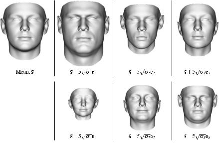
Fig. 4.1 A 3D morphable model of human faces [48]. The top left panel shows the mean face surface. The remainder show the mean face deformed by ±5 standard deviations along the first three principal modes of variation

a representation is that the high dimensional mesh can be approximated by the low dimensional parameter vector. Moreover, the parameter space is useful for recognition and classification and the modes themselves often correspond to meaningful global descriptors. For example, in Fig. 4.1, we show a morphable model of human faces. The first mode appears to capture the difference between adult and child faces. A morphable model is limited to representing objects from within the same class as the training data. The ability of the model to generalize to unseen samples is characterized by the generalization error, which is a function of the diversity of the training samples. There is also an implicit assumption that the original high dimensional data approximates a Gaussian distribution (hyperelliposoid), which can be accurately approximated by a small number of axes.

4.2.2.5 Implicit Surface

An implicit surface [8] (also known as a level set or an isosurface) is the set of all points [x y z]T which satisfy the function f (x, y, z) = 0. Typically, function values greater than zero indicate points that are outside the object, while negative values indicate points that are inside. For example, the surface of a sphere of radius r can be represented by the set of points satisfying x2 + y2 + z2 − r2 = 0. The surface normal to an implicit surface can be obtained simply by taking partial derivatives:

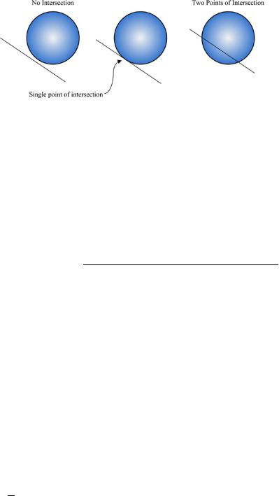
Fig. 4.2 The three possible cases for a line-sphere intersection

Inside/outside tests can also be performed efficiently by simply evaluating the sign of the surface function at a given point. One of the most attractive properties of the implicit surface representation is that intersections can be computed analytically. By substituting a parametric ray equation into the implicit surface function and solving for the parameter, all intersections can be found exactly. For example, consider the ray described by:

Substituting into the parametric surface for the sphere, radius r , given above yields:

(4.4) There are three possible cases for this intersection (see Fig. 4.2). Two real roots means that the ray intersects the sphere in two places. One real root means the ray touches the sphere tangentially. No real roots means the ray misses the surface. Higher order surfaces involve the solution of higher order intersection equations, which may not be possible analytically.

In general, obtaining a function which exactly describes a general surface is difficult. However, for applications involving visualization of physical effects such as fluid dynamics (where functional descriptions of the dynamics are readily available) an implicit surface is a natural representation. There are a number of commonly used ways to define an implicit surface. The example above is algebraic. The most common such form is a quadric which can be used to describe regular shapes such as spheres, ellipsoids and tori.

An alternative is to derive an algebraic representation from an intermediate representation [9], which is specified by a designer or fitted to data. The most common approach is to define a control structure from primitives such as points, line segments and planar patches. A field function is defined and its value at some point is determined by the distance, r , from that point to a control structure. For example: f (r) = r12 . The value of this function is known as the field strength. The total field

strength is the sum of the field strengths due to each control structure. Distances to line segments and planes is usually taken as the distance to the closest point on the structure. A single point yields a sphere whose radius is determined by the chosen contour value. Where there are more than one control point, the fields interact and the resulting isosurface bulges between points. Approaches along these lines are known variously as metaballs, blobbies and soft objects. Rendering isosurfaces for display is not straightforward. The most common approach is to convert to a polygonal model [7]. Alternatives include raytracing the surface [21], which involves computing ray-surface intersections, as described above, or using point sampling and point-based rendering. An implicit surface representation that is commonly used for the interpolation of ‘missing parts’ of surfaces is the Radial Basis Function [11].

4.2.2.6 Parametric Surface

A parametric surface [14] is one which is defined by parametric equations with two parameters, as follows:

x = fx (u, v),

y = fy (u, v),

z = fz(u, v).

For example, the radius r sphere example given above can be described in terms of spherical coordinate parameters:

x = r sin θ cos α,

y = r sin θ sin α,

z = r cos θ .

A surface in such a form is easy to evaluate and, if the parametric equations are differentiable, it is straightforward to calculate differential properties of the surface. The problem is that it is very difficult to describe anything other than fairly simple shapes using an algebraic parametric description. For this reason, complex shapes are composed from piecewise parametric surfaces. These parametric patches are blended together to obtain the overall surface and each patch is defined in terms of a set of control points over the unit square. To evaluate a parametric patch at a point, the tensor product of parametric curves defined by the control points is computed. This is achieved by combining control points with polynomial blending functions. Most commonly, these are bicubic:

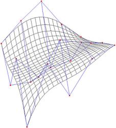
Fig. 4.3 A Bézier surface patch. Control points are shown in red, the control grid in blue and the interpolated surface in black

where U = [u3 u2 u 1] and V = [v3 v2 v 1] and

are the function values of the control points (for a bicubic patch, these are specified by a 4 × 4 grid sampling). The matrix M describes a blending function for a parametric cubic curve. Two common examples include B-spline:

Bézier patches have some useful properties. The patch will lie completely within the convex hull of its control points and the Bézier surface will pass through the control points at the corner of the patch. It does not generally pass through the other control points. They are visually intuitive and popular in interactive editing applications for this reason. An example of a Bézier patch is shown in Fig. 4.3. To achieve C0 continuity between adjacent patches, the boundary control points (and