Материал: [2.1] 3D Imaging, Analysis and Applications-Springer-Verlag London (2012)

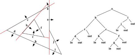
Fig. 4.8 A 2D example of a Binary Space Partitioning tree

and branching at nodes representing the outcome of the binary test. This is a simple and elegant representation on which boolean operations and point classifications are easy to compute, though it potentially results in a high memory overhead. The representation was first proposed by Fuchs et al. [16] and is a popular representation in graphics, where calculation of visible triangles from arbitrary viewpoints is required.

In Fig. 4.8, we provide an example of a BSP tree. In this case, the tree operates in 2D and hence the binary tests determine which side of each line a point lies and the resulting object is a 2D area.

4.2.3.4 Constructive Solid Geometry

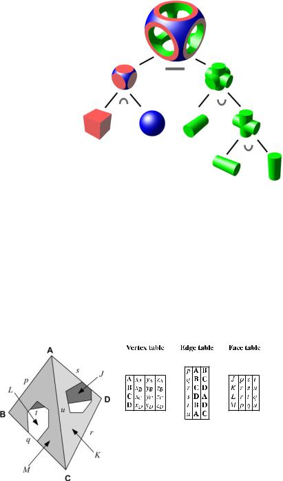
Constructive Solid Geometry (CSG) [34] is a representation for solid objects based on compositions of simple primitive solids. They are combined using boolean set operations. The primitives and operations can be stored efficiently in a binary tree in which the leaves contain primitives, nodes contain operators and the represented object lies at the root. Figure 4.9 shows an example of a complex solid constructed from a small number of primitives and operations. The CSG representation is intuitive and relates well to CAD interfaces. However, representing arbitrary solids in this way can prove inefficient. In the context of 3D imaging, CSG can be useful for applications with “humans in the loop”. For example, in content-based retrieval, a human must be able to construct a coarse 3D model with which to search. Another example is fitting a part-based model to 3D data (such as body parts to human motion data). In this case, the parts can be constructed by a human using CSG. Finally, for indexing 3D data, a very low-dimensional description of an object can be obtained by fitting a CSG model to the 3D data and determining similarity by comparing CSG trees.

4.2.3.5 Boundary Representations

Boundary representations (known as B-reps) [65] describe solids by defining the boundary between solid and non-solid. They are widely used in Computer Aided

4.2.4 Summary of Solid-Based Representations

The method of acquisition of 3D data determines in which of the raw representations the data is delivered. Although some operations are possible on such data (for example, point-based rendering of point clouds), most applications necessitate conversion to a higher level representation. This may require a degree of approximation, for example, integrating a depth map from surface normal data.

The choice between surface-based and solid-based representations is dictated by the nature of the data and the intended application. On the other hand, certain representations are amenable to creation and editing by hand, for example by an animator or CAD designer. The requirements here may include ease and intuition of editing operations and guarantees about the nature of the resulting surface, such as smoothness. Other factors which may influence the choice of representation include storage and processing efficiency, representational power (e.g. some representations can only describe surfaces which are manifold or continuous) and the efficiency with which the representation can be rendered for visualization.

4.3 Polygon Meshes

Polygonal meshes are of such importance and are used so ubiquitously throughout computer graphics and computer vision that we provide a more in depth discussion of the file formats and data structures available for their storage and representation. We focus particularly on triangular meshes, though the representations extend naturally to quad or arbitrary polygon meshes.

Formally, a triangular mesh of N vertices is defined as a pair: M N = (KN, S). The topology, or connectivity, of the mesh is given by the simplicial complex KN, which is a set whose elements can be vertices {i}, edges {i, j } or triangles {i, j, k},

with the indices i, j, k [1 . . . N ]. The actual shape of the mesh is given by the vector S R3N , where the ith vertex is given by vi = [S3i−2 S3i−1 S3i ]T . There is

some redundancy in this representation (for example, edges can be inferred from triangles) and so not all representations store all of this information.

4.3.1 Mesh Storage

There are a wide range of open and proprietary file formats for the storage of mesh data. These can be categorized into binary and ASCII text formats. The former are more space efficient while the latter are human readable and editable. In general, these file formats all comprise a list of 3D vertices followed by a list of polygons which index into the vertex list. The files may also store vertex or face attributes such as surface normals and texture coordinates.

The most commonly used text-based formats are OBJ (originally developed by Wavefront Technologies) and VRML (Virtual Reality Modeling Language), which

was designed particularly with the World Wide Web in mind. The most popular binary format is 3DS which has grown to become a de facto industry standard for transferring models between 3D programs. As well as 3D data, this format can also include scene properties such as lighting. Finally, the PLY format (developed at the Stanford Graphics Lab) supports both ASCII and binary storage.

As the most frequently used format for model archiving, we briefly describe the OBJ format. This is composed of up to four parts, two of which are required. The following snippet provides an example OBJ file:

#Vertex (x,y,z) coordinates v 0.123 0.456 0.789

v ...

...

#Texture coordinates (u,v) coordinates vt 0.500 0.600

vt ...

...

#Normals in (nx,ny,nz) form

vn 0.707 0.000 0.707

vn ...

...

# Face Definitions f 1 2 3

f 3/1 4/2 5/3

f 6/4/1 3/5/3 7/6/5 f ...

...

Comments can appear anywhere within the file and are indicated by the line beginning with a hash symbol. The file must begin with a list of 3D vertex positions. Each is entered on a separate line, starting with “v”. Then there are two optional parts: 2D texture coordinates (line begins with “vt”) and 3D vertex normals (line begins with “vn”). Texture coordinates are 2D coordinates in the range [0, 1], which index into a texture map (which is typically square). Texture coordinates are scaled by the dimensions of the texture map and color values interpolated from the pixels surrounding the scaled texture coordinate position. The vertex, texture coordinate and surface normal lists should be of the same length. Texture coordinates and normals are assigned to the vertex in the corresponding position in the vertex list. The final required part comprises face definitions. Each face definition can take four possible forms, as follows:

Vertex. A valid vertex index starts from 1 and indexes into the previously defined vertex list. Faces may have more than three vertices.

f v1 v2 v3 v4 ...

Vertex/texture-coordinate. A vertex index may be followed by a texture coordinate index, separated by a slash.

f v1/vt1 v2/vt2 v3/vt3 ...

Vertex/texture-coordinate/normal. A vertex index may be followed by both a texture coordinate and surface normal index, each separated by a slash.

f v1/vt1/vn1 v2/vt2/vn2 v3/vt3/vn3 ...

Vertex/normal. A vertex index may be followed by only a surface normal index, separated by a double slash.

f v1//vn1 v2//vn2 v3//vn3 ...

An OBJ file may be augmented by a companion MTL (Material Template Library) file, which describes surface shading and material properties for the purposes of rendering.

4.3.2 Mesh Data Structures

To apply any processing to a mesh, such as rendering, manipulation or editing, we must be able to retrieve elements of the mesh and discover adjacency relationships. The most common such queries include: finding the faces/edges which are incident on a given vertex, finding the faces which border an edge, finding the edges which border a face, and finding the faces which are adjacent to a face. Mesh data structures can be classified according to how efficiently these queries can be answered. This is often traded off against storage overhead and representational power.

There are a large number of data structures available for the purpose of representing meshes. Some of the most common are summarized below.

Face list. A list of faces, each of which stores vertex positions. There is no redundancy in this representation, but connectivity between faces with shared vertices is not stored. Adjacency queries or transformations are inefficient and awkward.

Vertex-face list. A commonly used representation which is space efficient. It comprises a list of shared vertices and a list of faces, each of which stores pointers into the shared vertex list for each of its vertices. Since this is the representation used in most 3D file formats, such as OBJ, it is straightforward to load archival data into this structure.

Vertex-vertex list. A list of vertices, each containing a list to the vertices to which it is adjacent. Face and edge information is implicit and hence rendering is inefficient since it is necessary to traverse the structure to build lists of polygons. They are, however, extremely simple and are efficient when modeling complex changes in geometry [61].

Edge list. An edge list can be built from a vertex/face list in O(M) time for a mesh of M faces. An edge list is useful for a number of geometric computer graphics algorithms such as computing stencil shadows.