Материал: [2.1] 3D Imaging, Analysis and Applications-Springer-Verlag London (2012)

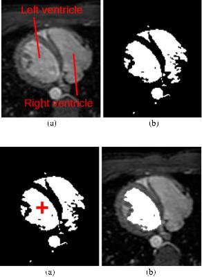
Fig. 11.13 Thresholding an axial cardiac MRI slice.

(a) Original slice. (b) Result of thresholding operation

Fig. 11.14 Segmenting the left ventricle using region growing on the thresholded axial cardiac MR slice.

(a) Thresholded image with seed point in the left ventricle indicated by the red cross. (b) Result of region growing, overlaid onto original cardiac MRI slice

11.5.1.2 Region Growing

One technique that can be used to refine thresholded images, such as that shown in Fig. 11.13b, is known as region growing. Region growing involves user interaction in the form of specifying a seed point. This is a pixel in the image that is known to lie inside the structure being segmented. The region is then iteratively grown by adding neighboring pixels that have similar appearance. The concept of similarity needs to be defined: for example, by specifying a range of intensity values around that of the seed pixel. If region growing is applied to a thresholded image then, to be considered similar, pixels should have the same binary value as the seed pixels. In addition, the concept of neighborhood needs to be defined, with 4-neighborhoods (i.e. only directly adjacent pixels) and 8-neighborhoods (i.e. including diagonally adjacent) commonly used in 2D images. Figure 11.14 illustrates the operation of the region growing algorithm for segmenting the left ventricle from the cardiac MRI data introduced in Fig. 11.13. A seed point has been placed in the left ventricle (indicated by the red cross) and the region growing algorithm has included all pixels that were connected to this seed, excluding all others. The resulting segmentation is of the left ventricle only.

Algorithm 11.1 REGION GROW on seed pixel Require: Initialize all pixels to unknown region

Set current pixel to be inside region for all neighboring pixels do

if it is inside image bounds and currently has an unknown region then Compute similarity to current pixel

if similar then

REGION GROW on neighboring pixel else

Set neighboring pixel to background end if

end if end for

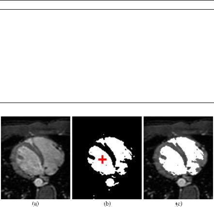
Fig. 11.15 The problem of leaks in region growing. (a) An axial cardiac MRI slice. (b) Result of thresholding operation, seed point for region growing in the left ventricle indicated by the red cross. (c) Result of region growing. The segmentation has ‘leaked’ into the right ventricle

The region growing algorithm can be implemented in a number of ways. The simplest, although not the most computationally efficient, is a recursive implementation. There are many implementations and this is the same problem as flood-fill or area-fill in graphics or vision. Pseudocode for recursive region growing is given in Algorithm 11.1.

One problem that the region growing algorithm can encounter is that of leaks. This problem is illustrated in Fig. 11.15. This shows a different axial cardiac MRI slice from that used in Fig. 11.13 and Fig. 11.14. This time the region growing has ‘leaked’ the segmentation into the right ventricle. Therefore, in region growing, care must be taken when selecting threshold values and specifying the similarity term to avoid such cases. The region growing algorithm can be extended to 3D, in which case the neighborhood in Algorithm 11.1 will extend to 3D accordingly. However, in 3D the problem of leaks can be exacerbated.

11.5.1.3 Deformable Models

Both thresholding and region growing are relatively straightforward techniques that can be important steps in a segmentation pipeline. However, they work only using the intensities in the image and impose no constraints on the shape of the resulting segmented object. A more sophisticated class of techniques that do incorporate such constraints is known as deformable models [53]. Deformable models are contours (in 2D) or surfaces (in 3D) that move and deform according to an energy term. The energy term comprises two components:

•an internal energy, which typically constrains the contour/surface to remain approximately smooth with no sharp discontinuities, and

•an external energy, which pulls the contour/surface towards certain features in the image data, such as strong gradients.

The segmentation problem then becomes one of optimizing the parameters of the contour/surface to minimize the energy.

Deformable models come in many different forms, but they can be broadly split into two types: parametric deformable models and geometric deformable models. In parametric deformable models the contour/surface is explicitly parameterized, for example by specifying a set of control points between which a contour is interpolated. We describe in more detail two of the more popular parametric techniques below. In geometric deformable models, the contour/surface is defined implicitly. An example of such an approach is the ‘level set’ technique [33, 50], in which a 2D contour is defined as the zero-crossing of a signed 2D function. In this case, it is the function that is parameterized and the contour is encoded implicitly in this parameterization. Examples of the use of level sets in medical imaging include segmentation of brain images from MRI [2], segmentation of the left ventricle of the heart from MRI and ultrasound [60] and segmentation of the cerebral vasculature from CT angiography [51].

Snakes One of the most famous examples of a parametric deformable model is known as Active Contour Models or Snakes [40]. In the Snakes algorithm, the user initially defines an approximate contour for the object being segmented. The algorithm refines this contour by minimizing the energy term. Formally, if a 2D contour is defined by v(s) = [x(s), y(s)] with s varying between 0 and 1, the energy is defined as:

The internal and external energy terms Eint and Eext must be defined to suit the particular application. For example, how does the object appear in the image data? If the object’s boundary is defined by a strong gradient in the image then Eext should be high in cases where the Snake does not overlay such gradients. Similarly, Eint will be high for contours which have sharp changes in direction and low for smooth contours. Once these terms have been defined, an optimization strategy such as gradient descent is employed to iteratively adjust the contour definition to minimize the

Algorithm 11.2 SNAKES

Require: Initialize contour parameters i = 0

Compute energy at iteration 0: Esnake,0 repeat

Compute gradient of energy term Esnake,i Modify contour parameters to minimize energy i = i + 1

until Esnake,i − Esnake,i−1 < ε or maximum iterations reached

energy, Esnake. Fast implementations of the Snakes algorithm have been proposed that have a computational complexity of O(nm), where n is the number of control points and m is the size of the neighborhood in which the points can move [82].

There are several variants of the Snakes algorithm and the precise implementation details will depend on the choice of optimization strategy and the nature of the contour parameterization. However, pseudocode for a generic version of Snakes is given in Algorithm 11.2. In general, snakes work well where there are clearly defined edges in the image and the shape of the object is reasonably smooth, since sharp edges will be smoothed out by the snake’s internal energy, which resists high curvature. Finally, they can be interactively manipulated towards the edge of choice in semi-automatic applications. Examples of the use of Snakes for 2D medical image segmentation include segmentation of intra-vascular US [85] and annotation of specular masses from mammography images [56].

Balloons The original work on Snakes was designed for 2D image segmentation. A similar concept can be extended to 3D images. The 3D balloons technique [19] is one such example. This algorithm is illustrated in Fig. 11.16, which shows a 3D segmentation of the left ventricle from an MRI image, implemented in ITKSNAP (the 3D MRI image is the same image that the 2D slices in Figs. 11.13, 11.14 and 11.15 were extracted from). This shows how the internal energy term of the 3D balloons algorithm can constrain the shape of the segmented object to avoid the problem of leaks that we saw in Fig. 11.15. Each screenshot shows the current segmentation in red overlaid onto sagittal (top left), coronal (top right) and axial (bottom right) views through the MRI image, together with a rendering of the current segmentation (bottom left). The axial slice shown is the same slice used in Fig. 11.15, although the 3D segmentation operated on all slices in the MRI volume. The user initializes the segmentation by placing a ‘balloon’ (a spherical surface) inside the structure to be segmented, as shown in Fig. 11.16a. The algorithm then iteratively ‘inflates’ the balloon (see Fig. 11.16b, c) until it is stopped by forces based on the image data (see Fig. 11.16d). In the example in Fig. 11.16 the inflation of the balloon is stopped by the intensity gradient where the bright intensities of the left ventricle are next to the darker intensities of the surrounding myocardium. This iterative optimization works in a similar way to the original 2D Snakes technique. 3D balloons have been used for cardiac segmentation from US data [42] and cerebral cortex segmentation from MRI images [83].