Материал: [2.1] 3D Imaging, Analysis and Applications-Springer-Verlag London (2012)

11.4.2.2 Surface-Based Registration

Rather than using 3D points, one could imagine a registration based on linear features, such as blood vessels or ridges on the surface of an object. In practice, such registrations are rare and it is more common to use surfaces. This approach was first proposed for medical imaging by Pelizzari et al. [61] as the head and hat algorithm. This led to a number of techniques to register 3D images using distance maps, or chamfer maps, which are images showing the distance to a given surface. These techniques have been very much taken over by intensity-based registration for fully 3D volumes, but there is still a place for surface matching in image-guided surgery, which we will discuss later, and in situations where an accurate segmentation of two images has been created. The surface may be a polygonal surface or a set of surface points, but typically the preoperative surface will be triangulated and intraoperative measurements will be points. A surface-based similarity measure can be generated as the sum-of-squared distance from the surface points to the nearest points on the triangulated surface.

11.4.2.3 Intensity-Based Registration

One of the most successful methods in medical image registration in the last few decades has been the use of intensity-based similarity measures. Given that we have a transformation T from image IA(x) to image IB (y), we are able to calculate corresponding voxel intensities. For a given voxel at position x in image IA(x) the corresponding point in image IB will be IB (T(x)). We can now start to calculate some image statistics in the region of the overlap, , between the two images.

For example, if we are trying to register images from the same modality and patient, we could assume that corresponding voxels will have the same intensity. This means that, at registration, all voxels should be equal and we can minimize a cost function, CSSD, to give:

where N is the number of voxels in the overlap. This is simply the mean sum of squared differences of intensities between the images. Thus, by minimizing CSSD(T) over the parameters of our transformation, T, we can achieve registration without needing to extract landmarks.

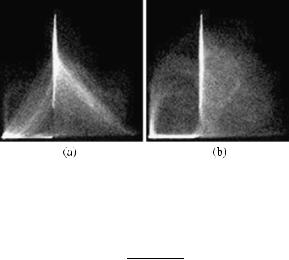
If we know the voxel intensities of the two images are an increasing function of each other, but we can’t be sure that they have the same intensities, then perhaps cross-correlation would be a more appropriate measure. When the relationship between intensities in the two images is not known we can use information theoretic measures to provide a similarity measure. We start by producing a 2D histogram. For each corresponding pixel we have an intensity IA and an intensity IB . These form a point on a graph of intensity in image type A (CT, say) vs image type B (MRI,

Fig. 11.11 MR vs CT joint histogram—at registration (a) and misregistered (b). The bright vertical line corresponds to soft tissue (large variation in MR, little in CT)

say). By choosing appropriately sized bins, we can form a probability distribution p(A, B), which is described by the joint histogram (see Fig. 11.11).

Mutual information (MI) can now be calculated as:

AB

where p(A, B) is the probability of a pixel having intensity A in the first image and intensity B in the second image and p(A), p(B) are the marginal probabilities that a pixel has a given value in each separate image. In practical applications MI, and a normalized version (NMI) [75], have proven to be highly robust as a means of registering 3D medical images for rigid and non-rigid applications.

11.4.3 Registration Optimization

There are many optimization strategies that can be employed to calculate the registration. In general, we will have a cost function that can be calculated over the degrees of freedom of the transformation. In the case of point-based rigid registration, there is an analytic solution that can be solved either by singular value decomposition (SVD) or by quaternion methods [28]. The general problem of calculating a rotation given a set of corresponding points is known as the Procrustes problem. This rather disingenuous term refers to a character from Greek mythology, who would stretch or cut the limbs of his guest to make them fit the bed. This originally referred data being fitted to a model when there was no real relationship but the term is still used to refer to the respectable problem of shape alignment.

For surface matching, there is the simple algorithm known as iterative closest points (ICP) [10]. Here, we have a set of points xi on one surface and we find the closest points y0i on the other surface. The next step in the algorithm is a standard rigid registration on the two point sets. After this, a new set of nearest points y1i is calculated and a new transformation calculated. After each iteration of this twostage cycle, the error between the data sets is reduced and will rapidly converge to a local minimum, which may or may not be a global minimum. The method

requires computation of nearest points on a surface, which can be made much more efficient using data structures such as k-d trees [8]. It should be mentioned that surface registrations such as this are very prone to multiple local minima (i.e. that are not globally minimal). Thus, depending on the starting alignment, the algorithm may get stuck an undesired local minimum. A combination of landmark and surface registration may be better behaved in terms of this problem. ICP and other methods of surface registration are discussed in more detail in Chap. 6.

For any type of non-linear transformation and for rigid or non-rigid intensitybased registration, the solution must be calculated iteratively. A hierarchical coarse- to-fine approach aids smoothness and convergence. A technique known as Parzen windowing can be used to estimate gradients in the cost function [79]. There are potentially a large number of parameters to optimize with intensity-based non-rigid registration (three times the number of control points) and registrations can take several hours. Various implementations incorporating GPU calculations have been proposed to speed up this process and efficient intensity-based non-rigid registration is the subject of ongoing research.

11.4.3.1 Estimation of Registration Errors

In all cases of registration, it is important to consider the problem of error estimation. Again, for the simple case of isotropic errors in point-based registration, an analytic solution is given by Fitzpatrick [28]. This relates the expected squared value of target registration error, TRE2(r) , (at some target point, r, other than the fiducials used to register) to the expected squared value of the fiducial localization error, FLE2 , (the error at which individual fiducials are localized) as follows:

where N is the number of fiducials, dk is the distance from the target point to the kth principal axis of the fiducials, and fk is the RMS distance of the fiducials to the same axis. The second term in brackets is similar to a moment-of-inertia. The centroid is the most accurately located point and rotational errors mean that TRE increases further away from the principal axes. This equation tells us that not only an increase in the number of fiducials improves the registration error, but also their spread with respect to the principal axes. Any configuration of points that approaches being on a line can lead to significant rotational errors away from the fiducials even if the residual error is low.

For higher dimensional data, such as surfaces, there is no analytic solution for the errors. Experience tells us that surface registration can be unreliable and should not be used alone without some validation or involvement of landmark data. In particular, surface registration is likely to fail if the surface shape has any rotational or translational symmetry or where there is non-rigid tissue motion. Intensity-based registrations have been used for many years and are found to be highly robust.