Материал: Russian Journal of Building Construction and Architecture

Russian Journal of Building Construction and Architecture

The operation of the well with filtration flows of underground water has been given particular consideration [12]. The Earth and the well have their own distinct features that need to be considered in a mathematical model. Firstly, a geothermal well is defined as a local source or sink of heat and basically it causes a local disruption of the global temperature field of the Earth (in case of heat supply) or a temperature drop (in case of heat removal) in the influence area of the well. After a heat pump stops, there is a gradual return to a background value. Secondly, a significant mass of soil massif and thermal resistance of a layer cause a considerable reduction in the influence area of the well decreasing the cooling or heating rate. In combination with small densities of background heat flows of a layer it is advisable to make use of a heat accumulator as well that operates more efficiently in a sign-changing operation mode of a heat pump implanting heat regeneration. Thirdly, non-stationary operation mode of the well is due to the operation of heat pump as part of systems of heat supply or heat supplyconditioning where demand for heat depends on a variety of factors stemming from technology, hydrogeology or climatе. Fourthly, a filtration flow of underground water might have an influence on the operation of the well.

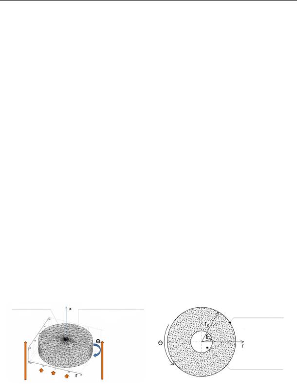
Mathematical modeling of a temperature field of a soil when geothermal energy is reduced to solving the problem of non-stationary thermal conductivity as in [17, 18, 20]. But in this case in order to design a model a cylindrical coordinate system that considers a background heat flow of the Earth to its surface was chosen (Fig. 2).

Fig. 2. Model of an operated soil massif:

а) general view; b) top view;

rк is the radius of a boring column, m; rс is the radius of the well, m; Qфон is the background flow of the Earth, Watt/m2

40

A feature of the problem is non-stationary heat exchange that is caused by multiple alternating cycles of switching on a system of heat supply – conditioning with seasonal reverses of heat flow and switching it off [14].

where t is the temperature of a soil, 0С; τ is the time время, sec; a is the coefficient of temperature conductivity, m2/seс; r is a radial coordinate, m; qv are sources and sinks of heat influenced by heat flows of the Earth and heat emissions through the surface, Watt/m3; с is the heat capacity, J/(m3 С).

2. Boundary conditions for designing a model. The boundary conditions at the outlet of the well Tоси were accepted depending on the technological modes.

1. Operating conditions without changing the direction of a heat flow:

––at the boundary of the influence area of the well in the layer the first-order boundary conditions with a constant background temperature of a soil t ( , τ) = tфон are accepted;

––the second-order boundary conditions are specified on the surface of the boring column while the heat pump is operating:

t(rcr, ) qскв ,

while it is not operating:

t(rc , ) 0,

r

where qскв is the density of a heat flow on the surface of the boring column of the well determined with a heat load of the system of heat supply and conditioning;

–– there is a simplification that involves the second-order boundary conditions at the lower generating line of a design cylinder, background heat flow of the Earth is considered constant:

t(r, ) q ;r

–– on the surface of the Earth the third-order boundary conditions determined with climatic conditions and heat emission with a relatively small error can be replaced by the first-order boundary conditions: t (r, ) = tclimate. The assumption is made due to a considerably larger coefficient of heat emission on the surface compared to the coefficient of heat emission of the soil from the surface before the heat exchange part of the well.

41

Russian Journal of Building Construction and Architecture

2. The operating conditions of the heat supply/air conditioning system in the sign-changing mode differ in the reverse of the heat flow on the surface of the boring column:

t(rcr, ) qскв .

For a qualitative description of the ratio of the supplied and deflected amount of heat for a sign-changing technological mode the concept of the coefficient of heat regeneration kр is introduced that is given by the ratio of absolute values of the supplied and deflected heat:

where Qподвод is the amount of the supplied flow in the cold season, J; Qотвод is the amount of the deflected flow in the warm season, J.

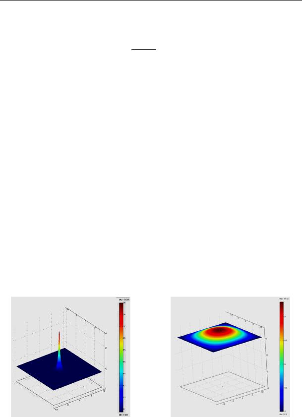
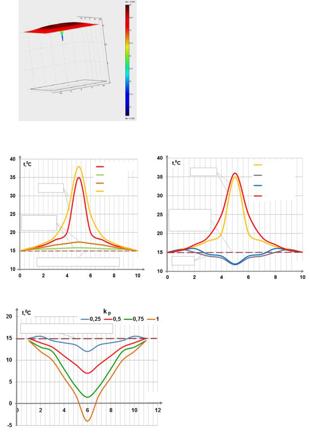
3. Results of the numerical experiments and natural studies. Unlike [16], the investigated numerical model is based on discrete representation of an energy equation, boundary and initial conditions but for different densities of a heat flow and it is implemented using the MathLab software package. Change in the temperature field for cyclic heat deflection into the well of 100 Watt/m2 is depicted in Fig. 3—4. The temperature of the soil layer of the well during one-flow mode from when the heat pump is first switched on increases rapidly and during the third year of the operation it becomes stable (Fig. 3а). During downtime (Fig. 3b) the temperature of the layer became equal and at the outlet of the well Tоси a deviation from the background temperature remained in the range of 2 С.

Fig. 3. Change in the temperature field:

а) аctive load during 6 months; b) downtime mode of the heat pump

42

c)

Background temperature of the layer

Fig. 4. Change in the temperature of the layer after the first switching until the quasi-stationary state is reached:

а) one-flow mode; b) sign-changing mode;

c) temperature graph of the layer at kр from 0 to 1

r, m

43

Russian Journal of Building Construction and Architecture

A quasi-stationary state that corresponds with a cyclic mode with no further increase in the temperature is reached at the stage after 2.5 years and during the downtime mode after 3 years (Fig. 4а). Compared to [1] changes in the temperature field when there is a reverse of the heat load on the layer (Fig. 4а, b) shows that during regeneration the quasi-stationary state is reached after 1.5 years.

4. Obtaining criteria dependencies. For possible distribution of the obtained results and their further use as generalizing dependencies the similarity theory was employed. The known criteria of similarity and criteria equations[19, 21] are not completely representative of the investigated phenomena. Therefore the following dimensionless complexes were used: the dimensionless active sink Q, dimensionless temperature θ. The temperature field is described with the dimensionless function with three dimensionless influencing parameters: f = [Fo, Θ, Q]. The task involves the identification of the single-valuedness condition. Therefore the structure of the equations should be changed and the generalizing criteria of similarity modified in particular:

–– the criterion Fo:

where а is the coefficient of thermal conductivity, m²/sec; τ is a typical time of change in the external conditions, seс; rc is a typical size of a body (the radius of a well), m;

–– active dimensionless heat flow:

where qнагр is a specific reduced per an area unit of the boring column heat load on the well in a certain operating period, Watt/m2; qземли is the background heat flow of the Earth, Watt/m2; –– the dimensionless temperature:

where tостаточноегрунт is the temperature of the soil in the investigated period,0С; tос is the average temperature of the environment of the investigated period,0С; tфоновоегрунт is the background value of the temperature of the soil, 0С.

The results of the calculation of the temperature at the bottom of the geothermal well Тоси as a function of the determining parameters in a dimensionless size are presented in Fig. 5.

44