Материал: Russian Journal of Building Construction and Architecture

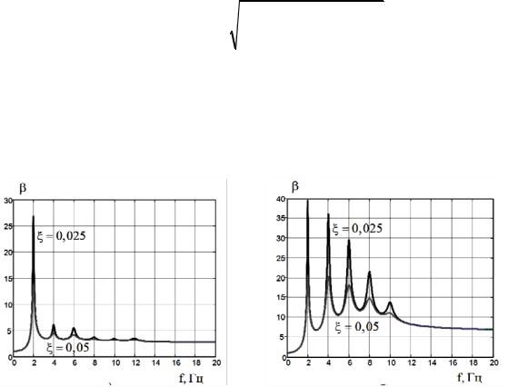
Fig. 2 shows the graphs of the dynamic factors in the axes of eigenfrequencies β(fk) at the impulse frequency fp=2 Hz: а) for pedestrian movement α = 2/3 and b) for high jumps α = 1/4; both graphs are designed for 5 % damping (the grey line) and 2,5 % damping (the black line).

Fig. 2

3. Quasi-static probabilistic solution

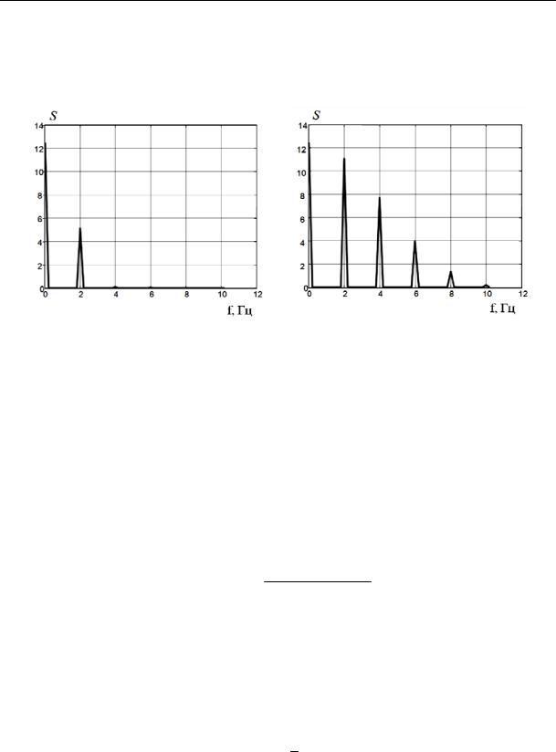
A random process corresponding to an impulse load is narrow, i.e. it is determined for a discrete set of frequencies nθ using the formula (2). The spectral density of the impulse load is functions close to the δ-function along the coordinates corresponding with the impact frequencies nθ, n =1, …, NF. Fig. 3 shows the graphs of spectral densities S, (kN/m2)2/Hz corresponding with the impulse loads in Fig. 1 at the impulse frequency fp = 2 Hz: а) for pedestrian movement α = 2/3, b) for high jumps α = 1/4.

In a temporary interval of active loading by a single impact a random process of spectator movement on a stand can be considered stationary, i.e. the average value and standard do not depend on time. The average value of a random process considering the ratios

Kp 2 , tp Tp

is

131

Russian Journal of Building Construction and Architecture

Therefore a load from the coordinated crowd movement can be considered as a stationary random process with an average value of that of a static load G.

where Q(t) is a stationary process at the input that corresponds with an external impact on the system; u(t) is a stationary process at the output that corresponds with a response (movement) of a system.

If a spectral density of a stationary process at the input SQ(θ) is known, a spectral density of a process at the output Su(θ) for a linear stationary system (10) is given by the formula [1, 2]

The concept of the dynamic factor is introduced similarly to determined established oscillations for harmonic loading. This factor shows by how many times a static load is to be increased so that dynamic effects are considered in the quasi-static approach.

Let us separate the constant multiplier G from the right part of the equation (10), which is an average value of a random load Q , then a generalized random force is

Q t GQ t .

Based on linearity of the system (10),

u t Gu t ,

132

where the random process u is movement from the force Q . Then due to stationarity of the

The dynamic factor β for random loads is determined as a ratio of the dynamic movement u to the static movement uG (i.e. the movement from the static load G):

The static movement uG does not depend on time and is determined using the equation (10) at

Q = G:

The final formula for the dynamic factors of the system with one degree of freedom is obtained using the equation (13) considering (14) and (15):

For multidimensional systems when a dynamic factor is different for oscillations along each k-th eigenfrequency, it is assumed to be a function of the eigenfrequencies Ωk:

This formula can be written using the modal damping coefficient k ( k k k ) and the frequencies expressed in Hz (SQ SQ f 2 , 2 f , k 2 fk ):

133

Russian Journal of Building Construction and Architecture

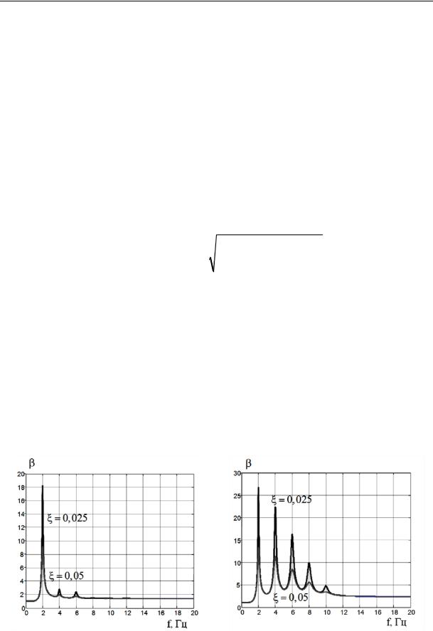
Fig. 4 shows the graphs of the dynamic factors β(fk) designed using the formula (16) for the frequency of the impulses fp = 2 Hz: а) for pedestrian movement α = 2/3 and b) for high jumps α = 1/4. The black line corresponds to 2.5 % damping, the grey line to 5 % damping.

4. Test calculation using a temporary range and result analysis

Based on the example of the system with one degree of freedom, we will consider how the quasi-static solutions described in Section 3 and 4 correlate with the test calculation in a temporary range. The formula (7) for the established movements of a one-mass system (10) is as follows:

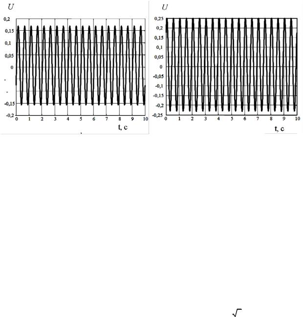
The test calculation is performed for a resonance mode when the frequency of an impulse load coincides with the eigenfrequency of the system: θ = Ω = 12.5664 rad/sec (2 Hz). Fig. 5 presents movements, m, as a time function, sec, for pedestrian movement (а) and high jumps (b) in the range of 10 seс.

The load G is assumed to be one. Using the graphs, let us determine the probabilistic and determined dynamic factors and compare them with the factors obtained in Section 2 (see Fig. 2) and Section 3 (Fig. 4).

134

um = ust = 0.0063, standard σu = 0.1152; for the frequency 2 Hz the determined efficiency coefficient is βdet = ua /um = 25.78, the probabilistic one βstoch = σu /um = 18.29. The corresponding values in the diagrams (see Fig. 2а, 4а): βdet = 26.79 (the error is 3.8 %), βstoch = 18.24 (the error is 0.3 %).

For high jumps: the amplitude of the oscillations ua = 0.2432, average value um = ust = 0.0064, standard σu = 0.1689; for the frequency 2 Hz the determined efficiency coefficient is βdet = ua /um = 38.00, the probabilistic one βstoch = σu /um = 26.39. The corresponding values in the diagrams (see Fig. 2b, 4b): βdet = 39.44 (the error is 3.7 %), βstoch = 26.69 (the error is 1.1 %). The test resuts are indicative of the two above approaches being correct.

Note that as shown in [5], for the impulse spectral density stoch det 1 2 0.707. This is due to the fact that βstoch is a standard of a random dynamic factor. The ratio βstoch/βdet will be dropping considering a random character of the load.

5. Evaluation of the spectators’ perception of vibrations

A human body is a viscoelastic system with its own frequencies. Resonance frequencies of certain body parts are as follows: [3]: eyes — 12—27Hz, throat — 6—27 Hz, chest — 2— 12 Hz, legs and arms — 2—8 Hz, head — 8—27 Hz, face and jaw — 4—27 Hz, lumbar spine — 4—14 Hz, stomach — 4—12 Hz. For the oscillation frequencies close to the resonance ones vibrations might have a range of negative impacts from unpleasant sensations to

135