Материал: Кластеризация данных. методические указания к выполнению практических работ для студентов направления 09.04.03 «Прикладная информатика». Головинский П.А., Шаталова А.О
from sklearn.cluster import KMeans from sklearn.datasets import make_blobs
plt.figure(figsize=(12, 12))
n_samples = 1500 random_state = 170
X, y = make_blobs(n_samples=n_samples, random_state=random_state)
# Incorrect number of clusters
y_pred = KMeans(n_clusters=2, random_state=random_state).fit_predict(X)
plt.subplot(221)
plt.scatter(X[:, 0], X[:, 1], c=y_pred) plt.title("Incorrect Number of Blobs")
# Anisotropically distributed data
transformation = [[0.60834549, -0.63667341], [-0.40887718, 0.85253229]] X_aniso = np.dot(X, transformation)
y_pred = KMeans(n_clusters=3, random_state=random_state).fit_predict(X_aniso)
plt.subplot(222)
plt.scatter(X_aniso[:, 0], X_aniso[:, 1], c=y_pred) plt.title("Anisotropicly Distributed Blobs")
# Different variance
X_varied, y_varied = make_blobs(n_samples=n_samples, cluster_std=[1.0, 2.5, 0.5], random_state=random_state)
y_pred = KMeans(n_clusters=3, random_state=random_state).fit_predict(X_varied)
plt.subplot(223)
plt.scatter(X_varied[:, 0], X_varied[:, 1], c=y_pred) plt.title("Unequal Variance")
# Unevenly sized blobs
X_filtered = np.vstack((X[y == 0][:500], X[y == 1][:100], X[y == 2][:10])) y_pred = KMeans(n_clusters=3,
random_state=random_state).fit_predict(X_filtered)
plt.subplot(224)
16
plt.scatter(X_filtered[:, 0], X_filtered[:, 1], c=y_pred) plt.title("Unevenly Sized Blobs")
plt.show()
____________________________________________________________________
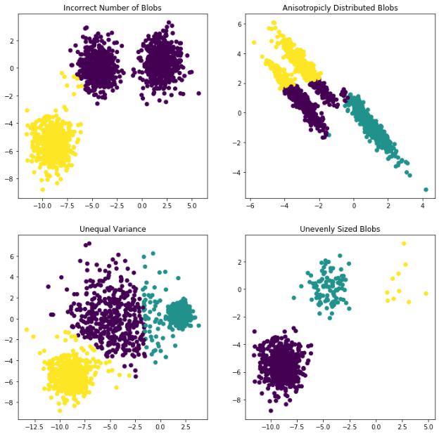
На рис. 5 представлены результаты работы программы кластеризации для разных наборов данных.
Рис. 5. Результаты кластеризации для разных типов данных
17
7.ПРОГРАММА КЛАСТЕРИЗАЦИИ С ПОМОЩЬЮ КАРТ
КОХОНЕНА [8,9]
import time
import numpy as np import tensorflow as tf
import matplotlib.pyplot as plt class SOMNetwork():
def __init__(self, input_dim, dim=10, sigma=None, learning_rate=0.1, tay2=1000, dtype=tf.float32):
if not sigma:
sigma = dim / 2 self.dtype = dtype #constants
self.dim = tf.constant(dim, dtype=tf.int64)
self.learning_rate = tf.constant(learning_rate, dtype=dtype, name='learning_rate')
self.sigma = tf.constant(sigma, dtype=dtype, name='sigma')
self.tay1 = tf.constant(1000/np.log(sigma), dtype=dtype, name='tay1') self.minsigma = tf.constant(sigma * np.exp(-1000/(1000/np.log(sigma))),
dtype=dtype, name='min_sigma')
self.tay2 = tf.constant(tay2, dtype=dtype, name='tay2') #input vector
self.x = tf.placeholder(shape=[input_dim], dtype=dtype, name='input') #iteration number
self.n = tf.placeholder(dtype=dtype, name='iteration') #variables
self.w = tf.Variable(tf.random_uniform([dim*dim, input_dim], minval=- 1, maxval=1, dtype=dtype),
dtype=dtype, name='weights') #helper
self.positions = tf.where(tf.fill([dim, dim], True))
def feed(self, input):
init = tf.global_variables_initializer() with tf.Session() as sess:
init.run()
win_index = sess.run(self.__competition(), feed_dict={self.x: in-
put})
win_index_2d = np.array([win_index//self.dim.eval(), win_indexwin_index//self.dim.eval()*self.dim.eval()])
return win_index_2d
18
def training_op(self):
win_index = self.__competition('train_') with tf.name_scope('cooperation') as scope:
coop_dist = tf.sqrt(tf.reduce_sum(tf.square(tf.cast(self.positions - [win_index//self.dim, win_index-
win_index//self.dim*self.dim],
dtype=self.dtype)), axis=1))
sigma = tf.cond(self.n > 1000, lambda: self.minsigma, lambda: self.sigma * tf.exp(-self.n/self.tay1))
sigma_summary = tf.summary.scalar('Sigma', sigma)
tnh = tf.exp(-tf.square(coop_dist) / (2 * tf.square(sigma))) # topological neighbourhood
with tf.name_scope('adaptation') as scope:
lr = self.learning_rate * tf.exp(-self.n/self.tay2)
minlr = tf.constant(0.01, dtype=self.dtype, name='min_learning_rate')
lr = tf.cond(lr <= minlr, lambda: minlr, lambda: lr) lr_summary = tf.summary.scalar('Learning rate', lr) delta = tf.transpose(lr * tnh * tf.transpose(self.x - self.w)) training_op = tf.assign(self.w, self.w + delta)
return training_op, lr_summary, sigma_summary
def __competition(self, info=''):
with tf.name_scope(info+'competition') as scope:
distance = tf.sqrt(tf.reduce_sum(tf.square(self.x - self.w), axis=1)) return tf.argmin(distance, axis=0)
#== Test SOM Network ==
def test_som_with_color_data(): som_dim = 100
som = SOMNetwork(input_dim=3, dim=som_dim, dtype=tf.float64, sigma=3) test_data = np.random.uniform(0, 1, (250000, 3))
training_op, lr_summary, sigma_summary = som.training_op() init = tf.global_variables_initializer()
writer = tf.summary.FileWriter('./logs/', tf.get_default_graph()) with tf.Session() as sess:
init.run()
img1 = tf.reshape(som.w, [som_dim,som_dim,-1]).eval() plt.figure(1)
plt.subplot(121)
plt.imshow(img1) start = time.time()
for i, color_data in enumerate(test_data): if i % 1000 == 0:
19
print('iter:', i)
sess.run(training_op, feed_dict={som.x: color_data, som.n:i}) end = time.time()
print(end - start)
img2 = tf.reshape(som.w, [som_dim,som_dim,-1]).eval() plt.subplot(122)
plt.imshow(img2)
writer.close()
plt.show() test_som_with_color_data()
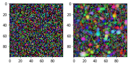
На рис. 6 приведены исходные данные (слева) и результат кластеризации по цветам (справа).
Рис. 6. Кластеризация по цветам
8.ПРАКТИЧЕСКИЕ ЗАДАНИЯ
1.Взять лист бумаги в клетку.
2.Получить от преподавателя набор данных на плоскости для кластери-
зации.
3.Выбрать одну из программных реализаций кластеризации [7] или [8] методом k-средних.
4.Выполнить кластеризацию и сделать выводы.
5.Установить в ANACONDA дополнительный пакет tesorflow.
6.Выполнить программу кластеризации изображения по цветам с помощью карт Кохоннена [9, 10].
7.Создать отчет в Word о выполненной практической работе с описанием исходных данных, промежуточных результатов работы программ, полученным результатам классификации и выводами.
20