Материал: Маслов ИНТРОДУЦТИОН ТО ПХЫСИЦС ОФ СЕЦОНД-ОРДЕР МАГНЕТИЦ 2015
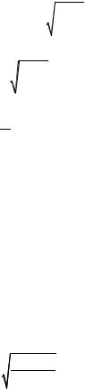
where α ≈ θa2, so that at
and thus
g(gR)
at R >> a. Designating
rewrite Eq. (25.24) as
J (q) =q−αq2 ,
T > θ from Eq. (25.11) we have
|
|
|
|
T |
|
|
|
|
|
|
|
|
|||
|
g(q) = |
|
|
|
|
|
|
|
|
||||||
|
T −q+ αq2 |
|
|
|
|
||||||||||
|
|
1 T a |
|
|
|
|
|
|
|
|
R |
||||
|
|
|
|
|
T |
−θ |
|||||||||
≈ |
|
|
|
|
|
exp |
− |
|
|
|
|
|
|
|
|
|
|
|
|
|
|
|
|
|
|
|
|||||
|
|
4p θ R |
|
|
|
|
|
|
|
|
|
|
|||
|
|
|
|
|
|
|
|
θ a |
|||||||
|
|
ξ = a |
|
θ |
|
, |
|
|
|
|
|
||||
|
|
|
T −θ |
|
|
|
|
|
|||||||
|
|
|
|
|
|
|
|
|
|
|
|
|
|
||
g(gR) − Ra exp(−R x).
x).
(25.22)
(25.23)
(25.24)
(25.25)
(25.26)
We see that the correlation function falls off exponentially with the distance R between two moments at a characteristic length ξ. This is why
ξ is called the correlation length or the correlation radius. Of fundamental importance is that ξ increases as T decreases and diverges as T → 0.
We turn to the case T < θ. At T = 0 from Eq. (25.20) one has g(R) =
= 1 for any R. At 0 < T < θ and R >> a the expression for g(R) takes the form
g |
2 |
|
1 T a |
|
|
R |
|
|
|||
g(R) ≈ x |
|
+ |
|
|
|
exp |
− |
|
|
, |
(25.27) |
|
4p θ R |
|
|||||||||
|
|
|
|
|
x |
|
|
||||
where the correlation length ξ is now
|
θ |
|
ξ = a |
2(θ−T ) . |
(25.28) |
It diverges at T → θ, as in the case T > θ.
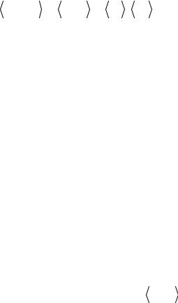
Finally we note that correlations of magnetic moments are intimately related to their fluctuations, the corresponding operators being
δσiz = σiz −  σiz
σiz  T :
T :
71
|
|
|
|
|
|
δ δ |
2 |
. |
(25.29) |
δσiz δσjz |
= σiz σjz |
− σiz |
σjz |
= g(Ri − Rj ) − x |
|||||
|
T |
|
T |
|
T |
T |
|
|
|
26. Heat capacity of a ferromagnet in the Ising model with account for fluctuations
For the contribution from local magnetic moments to the specific heat of a ferromagnet (that is, for the “spin component” of the specific heat) in the mean field approximation we had, see § 20:
0, |
T > θ; |
|
|
|
3 |
|
(26.1) |
Cs (T ) = |
kB N, T = θ. |
||
|
2 |
|
|
|
|
|
|
This contradicts the experiment that clearly points to the divergence of
Cs at T → θ.
Let us calculate Cs beyond the mean field approximation, with consideration for fluctuations of local magnetic moments, see § 25. By definition,
Cs (T ) = dEs (T ) . |
(26.2) |
dT |
|
where Es(T) is a component part of the total internal energy stemming from the subsystem of local magnetic moments. In the Ising model it is equal to the thermodynamic average of the model Hamiltonian, see Eq. (10.6):
Es (T ) = − |
1 |
∑ |
/ |
Jij |
|
(26.3) |
|
|
siz sjz |
||||
|
2 i, j |
|
|
|
T |
|
(we restrict ourselves to the case of zero magnetic field). Taking Eqs. (25.1) and (25.17) into account, one has
Es (T ) = − |
1 |
∑J (q)g(q) , |
(26.4) |
|
2 |
q |
|
where the function g(q) is temperature dependent.
Let us calculate Cs(T) in the very vicinity of the Curie temperature θ. Making use of expressions for g(q) at T > θ and T < θ, see § 25, evalu-
72
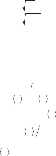
ating the sum over q in Eq. (26.4), and restoring the proper dimensionality, from Eq. (26.2) we have
|
|
|
|
|
|
|
|
|
|
|
|
|
|
θ |
|
, T |
|
> θ; |
|
|
|
|
|
|
|
|
|||
|
k |
|
T −θ |
||||||
Cs (T ) − |
B |
N |
|
|
|
(26.5) |
|||
|
|
|
|
|
|
|
|||
|
16π |
|
θ |
|
|
|
, T < θ. |
||
|
|
|
|
|
|
|
|
||
|
|
|
2(θ−T ) |
||||||
|
|
|
|
|
|||||
|
|
|
|
|
|
||||
Two equations (26.5) can be combined into a single one:
Cs (T ) − |
|
T −θ |
|
−0,5 at T → θ. |
(26.6) |
|
|
The critical exponent α = 0.5 in Eq. (26.6) differs from the experimental value α ≈ 0.1. Note however that accurate experimental determination of α is hampered by the sample inhomogeneity.
27. Magnetic susceptibility of a ferromagnet in the Ising model with account for fluctuations
Our purpose is to calculate the differential magnetic susceptibility
|
χ = ∂M (H ) ∂H , |
|
|
(27.1) |
||||||||
where |
|
|
|
|
|
|
|
|
|
|||
|
N |
|
|
|
NµB |
|
|
|
||||
M = |
µkz |
|
T |
= |
σkz |
|
|
(27.2) |
||||
|
|
|
|
|
T |
|
|
|||||
|
V |
|
|
|
V |
|
||||||
|
|
|
|
|
|
|
||||||
|
|
|
|
|
|
|
|
|
|
does not depend |
||
is the magnetization (we took into account that σkz T |
||||||||||||
on k). From Eqs. (27.1) and (27.2) one has |
|
|
|
|
|
|||||||
|
|
NµB2 |
|
|
|
∂h , |
|
|
|
|||
χ = |
|
|
|
∂ σkz T |
|
|
(27.3) |
|||||
V |
|
|
|
|||||||||
h = µBH. Recall that |
|
|
|
|
|
|
|
|||||
|
|
|
|
|
|
|||||||
|
Trσkz exp(−H / T ) |
|
|
|
||||||||
σkz T |
= |
|
|
|
|
|
|
|
, |
(27.4) |
||
|
|
|
|
Q |
|
|
||||||
where
73
|
|
1 |
N |
/ |
|
h |
N |
|
|
|
Q =Tr exp(−H |
/ T )=Tr exp |
|
∑ |
|
Jij σiz σjz + |
|
∑σiz |
(27.5) |
||
|
|
T |
||||||||
|
|
2T i, j=1 |
|
|
i=1 |
|
|
|
||
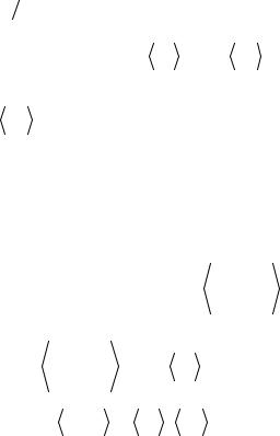
is the partition function. Taking in Eq. (27.5) the derivatives of both sides with respect to h/T, we have
|
∂Q ∂(h / T ) |
|
|
|
|
N |
|
|
|
|
|
|
|
|
|
|
|
|
|||||||||||||
|
=Tr∑σiz |
exp(−H / T )= |
|
|
|
||||||||||||||||||||||||||
|
|
|
|
|
|
|
|
|
|
|
i=1 |
|
|
|
|
|
|
|
|
|
|
|
|
|
|
|
|
||||
N |
|
|
|
|
|
|
|
|
|
|
N |
|
|
|
|
|
= NQ |
|
, |
|
|||||||||||
= ∑Trσiz exp(−H |
/ T )= Q∑ |
σiz |
|
|
σkz |
|
|||||||||||||||||||||||||
i=1 |
|
|
|
|
|
|
|
|
|
|
|
|
|
i=1 |
|
|
|
|
T |
|
T |
|
|||||||||
so that |
|
|
|
1 |
|
|
|
|
∂Q |
|
1 |
|
|
|
∂ln Q |
|
|
|
|
||||||||||||
|
|
|
|
|
|
|
|
|
|
|
|
, |
|
|
|
||||||||||||||||
|
|
|
σkz T = |
|
|
|
|
|
|
|
|
|
|
|
= |
|
|
|
|
|
|
|
|
|
|
|
|
||||
|
|
NQ |
|
∂(h / T ) |
|
|
N |
|
∂(h / T ) |
|
|
|
|||||||||||||||||||
and hence |
|
|
|
|
|
|
|
|
|
|
|
|
|
|
|
|
|
|
|
|
|
|
|
|
|
|
|
|
|
|
|
χ(H ) = |
µ2 ∂2 ln Q |
|
|
|
|
µ2 1 |
∂2Q |
|
|
1 |
∂Q |
|
2 |
||||||||||||||||||
B |
|
|
|
= |
|
|
|
B |
|
|
|
|
|
|
|
|
|
|
|
− |
|
|
|
|
|
|
. |
||||
VT ∂(h / T ) |
2 |
|
|
|
|
|
|
|
|
|
|
|
2 |
|
|
|
|
|
|||||||||||||
|
|
|
|
VT Q ∂(h / T ) |
|
|
Q ∂(h / T ) |
|
|||||||||||||||||||||||
|
|
|
|
|
|
|
|
|
|
|
|
|
|
|
|
|
|
|
|
|
|
|
|
|
|
|
|
||||
(27.6)
(27.7)
(27.8)
Now let us calculate the second derivative of Q with respect to h/T making use of Eq. (27.5):
∂2Q |
|
|
N |
|
2 |
|
|
N |
|
2 |
|
|
|
|
=Tr |
∑σiz |
exp(−H / T )= Q |
|
∑σiz |
. (27.9) |
|||||
∂(h / T ) |
2 |
|||||||||||
|
|
= |
|
|
|
|
|
= |
|
|
T |
|
|
|
i 1 |
|
|
|
i 1 |
|
|||||
From Eqs. (27.6), (27.8), and (27.9) one has
|
|
|
|
µB2 |
|
|
N |
2 |
|
|
N |
|
|
2 |
|
||||||
χ = |
|
|
|
|
|
|
|
∑σiz |
− |
∑ |
σiz |
|
|
|
= |
||||||
|
|
|
|
|
|
||||||||||||||||
|
|
|
VT |
i=1 |
|
T |
i=1 |
|
T |
|
|
||||||||||
|
|
|
|
|
|
|
|
|
|
|
|
|
|
|
|
|
|
|
|
||
|
|
|
µB2 |
|
|
N |
|
|
|
|
|
|
|
|
|
|
|
||||
= |
|
|
|
|
|
∑ |
|
σiz σjz |
− σiz |
σjz |
|
= |
|||||||||
|
|
|
|
|
|||||||||||||||||
|
|
|
|
|
|
|
|
|
|
|
T |
|
T |
|
|
|
|
||||
|
VT i, j=1 |
|
|
|
|
|
T |
|
(27.10) |
||||||||||||
|
|
|
|
|
µ2 |
|
|
|
|
|
|
|
|
|
|
|
|||||
|
|
|
|
|
|
N |
|
|
|
|
|
|
|||||||||
|
|
|
= |
|
|
B |
|
|
∑g(Ri |
− Rj ) − N 2 x2 |
|
= |
|
|
|||||||
|
|
|
VT |
|
|
||||||||||||||||
|
|
|
|
|
i, j=1 |
|
|
|
|
|
|
|
|
|
|||||||
|
|
|
|
|
|
µ2 |
|
|
|
N |
|
|
|
|
|
|
|
|
|||
|
|
|
= |
|
B |
|
N ∑g(q = |
0) − N 2 x2 |
. |
|
|
||||||||||
|
|
|
|
VT |
|
|
|||||||||||||||
|
|
|
|
|
|
|
|
R |
|
|
|
|
|
|
|
|
|||||
74
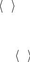
Making use of Eqs. (25.19) and (25.20) we arrive at
χ = |
µ2 |
1 |
at T > θ and T → θ, |
(27.11) |
||||||
B |
|
|
||||||||
VT T −θ |
||||||||||
|
|
|
|
|
||||||
χ = |
µ2 |
|
|
1 |
|
at T < θ and T → θ. |
(27.12) |
|||
|
B |
|
|
|
|
|
||||
VT 2(θ−T ) |
||||||||||
|
|
|
||||||||
Note that both these expressions do not differ from those derived in the mean field approximation, see § 21. Thus, account for fluctuations does not lead to qualitative changes in magnetic susceptibility.
28. Ising model for antiferromagnets. Mean-field approximation. Neél temperature
Up to this point we considered systems with exchange integral Jij > 0. As this takes place, the energy of the system is minimal if the
magnetic moments have the same direction like this ↑↑↑... ↑↑. And
what would happen if Jij < 0 ? Let us try to study this |
question. Again |
denote the Jij = J ( J < 0 ) for the nearest neighbors |
and Jij = 0 for |
other magnetic moments.
The beginning Hamiltonian will have the same form (see Eq. 10.7)
|
1 |
∑ |
/ |
|
|
(28.1) |
H = − |
|
|
Jij σiz σjz − h∑σiz . |
|||
|
2 i, j |
|
|
i |
|
|
Considering the mean-field approximation rewrite it in the following way
|
/ |
|
|
|
(28.2) |
H ≈ E0′ −∑ |
|
Jij σiz |
σjz |
−h∑σiz . |
|
i, j |
|
|
|
i |
|
Further, we shall leave out E0′
account for energy calculation obtaining. Finally receive
constant because it should be taken into but it is unimportant for order parameter
|
|
|
|
|
|
(28.3) |
H |
= −∑σiz h + ∑Jij |
σjz |
. |
|||
|
i |
|
i≠ j |
|
|
|
75