Материал: Маслов ИНТРОДУЦТИОН ТО ПХЫСИЦС ОФ СЕЦОНД-ОРДЕР МАГНЕТИЦ 2015
ond-order phase transitions are the ferromagnetic transition, superconducting transition, and the superfluid transition.
In this textbook, we outline the general features of second-order phase transitions by the specific examples of ferromagnetic and antiferromagnetic transitions in a solid state system of local magnetic moments. Author contributions: L.A. Openov wrote Preface, §§ 1–10, §§ 24–27; K.P. Katin and M.M. Maslov wrote §§ 11–23, §§ 28–30; M.M. Maslov coordinated all aspects of the work on this textbook.
1. Atomic magnetic moment
The net magnetic moment of every atom is determined by magnetic moments of constituting nucleus and electrons. Let us first make a rough estimate of the magnetic moment µ of a single atomic electron. Starting
with a classical equation
|
e |
|
|
|
µ = |
|
[rv |
], |
(1.1) |
2c |
where e, r , and v are, respectively, the electron charge, radius-vector, and velocity, and c is the speed of light, we have
m ~ |
| e |
| ap |
~ |
| e | |
~ 10-20 erg/G, |
(1.2) |
|
c |
m |
|
mc |
|
|
where a and p are characteristic values of, respectively, electron-nucleus separation and electron momentum, m is the electron mass, is the
Planck constant divided by 2π, and we made use of the Heisenberg uncertainty relation p ~ ħ/a.
More rigorous expression for µ follows from quantum mechanics. Since the classical relation between the magnetic moment of an electron
|
is, see (1.1), |
|
||
and its angular momentum M =[rp] |
|
|||
|
e |
|
|
|
m = |
|
M , |
(1.3) |
|
2mc |
||||
|
relates to the angular momentum op- |
|||
the magnetic moment operator µ |
||||
erator l as
6

|
e |
|
|
e |
|
|
|
|
|
|
|
|
|
|
|
m = |
|
M |
= |
|
l |
= −mB l , |
(1.4) |
2mc |
2mc |
where mB = |2emc| ≈ 9.974 10-21 erg/G is the so called Bohr magneton.
The operator of the magnetic moment projection on an arbitrary axis z is
|
|
(1.5) |
µz = −µB lz . |
||
For example, if an electron is in the state with an orbital quantum num-
ber l, then the quantum-mechanical eigenvalues of the operator lz (magnetic quantum numbers) are –l, –l + 1, …, l – 1, l. and hence possible magnetic moment projections µz are –µBl, –µB(l – 1), …, µB(l – 1),
µBl. In particular, µz = 0 for an electron occupying the symmetric s- orbital (l = 0).
Except an orbital angular momentum, every electron has an “intrinsic” mechanical angular momentum ħS, where S = 1/2 is the electron spin. As is shown in quantum electrodynamics, this results in the spin
magnetic moment µS whose operator is µS = −2µB S , so that the operator of the total electron magnetic moment becomes
|
|
|
|
|
|
|
(1.6) |
µ = −µB (l |
+ 2S ), |
||
and µz ≠ 0 even if l = 0.
The magnetic moments µi of all atomic electrons add up to give a net resulting magnetic moment of the atom µat , the corresponding operator being
|
|
|
|
|
|
|
ˆ |
|
|
|
|
|
(1.7) |
µat = ∑µi = −µB ∑(li |
+ 2Si |
)= −µB ∑(L |
+ 2S ), |
|||
|
|
i |
|
i |
i |
|
|
|
|||
|
|
and |
|
|
are the operators of the total electron |
where L |
= ∑li |
S |
= ∑Si |
||
|
i |
|
|
i |
|
angular momentum and total electron spin respectively (the contribution to µat from nucleus is negligible because of its large mass, see (1.2)). It
can be shown that L + 2S = g (L + S ), where g ~ 1 is the dimensionless Lande factor. For the sake of simplicity let us take L = 0 and S = 1/2. In
7

this case the operator of the atomic magnetic moment is (we omit the subscript “at”)
|
|
|
|
|
(1.8) |
µ = −gµB S , |
||
so that |
|
|
|
|
(1.9) |
µz = −2µ0 |
S z , |
|
where µ0 = gµB/2, and hence the z-component of the atomic magnetic
moment takes only two possible values, either +µ0 or –µ0. Such a moment is local in the sense that it is associated with a particular atom, being localized at that atom. In what follows, we shall consider macroscopic solid state systems of local magnetic moments.
2. Physical quantities characterizing the magnetic properties of matter
Any atom in the solid may carry a local magnetic moment µn , where n = 1, …, N is the number of a given atom and N 1 is the number of
atoms in the sample. The total magnetic moment is a vector sum ∑N µn
n=1
and depends on N. It is convenient to consider a specific magnetic moment called magnetization:
|
N |
V , |
(2.1) |
M = ∑µn |
|||
n=1
where V is the sample volume. In general magnetization can also result from electric currents flowing inside the sample.
As a rule (but not necessarily) magnetization arises upon application
of an external magnetic field of strength H and is linear in H at small
H:
Mα = ∑χαβHβ , |
(2.2) |
β |
|
where (α,β)= (x, y, z) and χαβ is the tensor of magnetic susceptibility.
In isotropic substance, χαβ = χδαβ , so that |
|
M = χH , |
(2.3) |
i.e., |
|
8

M = χH |
(2.4) |
for any direction in space. In the case that M is not linear in H, the differential magnetic susceptibility is used:
χ(H ) = ∂M (H ) ∂H . |
(2.5) |
Magnetic induction B (magnetic field in the sample) is the sum of external and induced fields:
B = H + 4πχM = µH , |
(2.6) |
where |
(2.7) |
µ =1+ 4πχ |
is the magnetic permeability.
3. Classification of materials for their magnetic properties
All materials (not only solids) may be categorized according to their magnetization M in an external magnetic field H :
1) nonmagnetic materials – M = 0 , i.e., B = H , χ = 0, µ = 1 (in an-
tiferromagnets, M = 0 as well, while the differential magnetic susceptibility is nonzero);
2) diamagnetic materials – |
M ↑↓ H , i.e., | B |<| H | (magnetic field |
||||||
in the sample is weakened), χ < 0, µ <1; |
|
||||||
|
|
1 |
|
|
|
||
3) superconductors – M = − |
|
|
H , i.e., B = 0 |
(magnetic field is ex- |
|||
4π |
|||||||
|
|
|
1 |
|
|||
pelled from the sample, Meissner effect), χ = − |
, µ = 0; |
||||||
4π |
|||||||
|
|
|
|
|
|
||
4) paramagnetic materials |
|
– |
|
M ↑↑ H , i.e., |
| B |>| H | (magnetic |
||
field in the sample is strengthened), χ > 0, µ > 1; |
|
||||||
5) ferromagnetic materials – |
M ≠ 0 at H = 0 , i.e., B = 4πM . In |
||||||
this case, the magnetic susceptibility defined by Eq. (2.3) is meaningless, while the differential magnetic susceptibility (2.4) makes sense. Ferromagnetism is observed only below the material-dependent Curie
temperature θ.
9
4. Isolated local magnetic moment in an external magnetic field
We consider an isolated local magnetic moment µ subjected to an
external magnetic field of strength H . In the case that this moment is associated with an atom in the solid, its kinetic energy is negligibly small, so that its total energy E is just an interaction energy U:
E =U = −µH , |
(4.1) |
|
and hence the Hamiltonian is |
|
|
|
|
|
|
(4.2) |
|
H |
= −µH , |
|
where µ is the magnetic moment operator. Taking a frame of reference with z-axis oriented along H , so that H = Hez , we have
|
|
|
|
|
H . |
|
(4.3) |
|
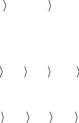
From Eq. (1.9) for µz |
|
H |
= −µz |
|
||||
we see that in the case S = 1/2 this operator |
||||||||
has two eigenstates, |
|
|
|
|
|
|
|
|
|
↑ |
|
0 |
and |
|
|
1 |
(4.4) |
|
|
|||||||
|
= |
|
|
↓ = |
|
|||
|
|
|
1 |
|
|
|
0 |
|
|
|
|
|
|
||||
corresponding to orientation of the magnetic moment along the z axis, i.e., along the applied field (“up”) and in the opposite direction (“down”) respectively. Note that the electron magnetic moment is antiparallel to the vector of its spin because of the negative electron charge.
|
|
in the states (4.4) are µz = µ0 |
and µz = –µ0, |
||||||
The eigenvalues of µz |
|
||||||||
µz |
|
↑ = µ0 |
|
↑ , µz |
|
↓ = −µ0 |
|
↓ , |
(4.5) |
|
|
|
|
||||||
where µ0 = gµB/2, see §1.
Since the Hamiltonian, Eq. (4.3), is linear in , the states (4.4.) are
µz
its eigenstates as well:
|
|
↑ = E↑ |
|
↑ |
|
|
↓ = E↓ |
|
↓ , |
(4.6) |
|
|
|
|
|||||||
H |
|
|
, H |
|
|
|||||
where |
|
E↑ = −µ0 H , E↓ = µ0 H . |
(4.7) |
|||||||
|
|
|||||||||
10