Материал: Маслов ИНТРОДУЦТИОН ТО ПХЫСИЦС ОФ СЕЦОНД-ОРДЕР МАГНЕТИЦ 2015

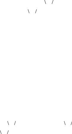
Внимание! Если размещение файла нарушает Ваши авторские права, то обязательно сообщите нам

This Hamiltonian has the same form as the Hamiltonian within the Ising model for ferromagnets. Earlier we denoted σjz = x (order parame-

ter). For every j these mean values σjz are identical due to the fact

that in ferromagnetic alignment all magnetic moments have the same direction. For antiferromagnets it will be different. For two neighboring

magnetic moments energy is equal to −J σiz σjz , and it has the minimal

			have different signs. In other
value if σiz σjz = −1, i.e.,	σiz	and σjz	have different signs. In other

words neighboring magnetic moments have different directions ( ↑↓). This applies for any pair of neighboring magnetic moments. What are our expectations? For one-dimensional case it will be like this:

↑↓↑↓↑↓... ↑↓. For two-dimensional simple cubic lattice the ordering is shown on Fig. 28.1.

↑↓↑↓↑↓↑↓

↓↑↓↑↓↑↓↑

↑↓↑↓↑↓↑↓

↓↑↓↑↓↑↓↑

Fig. 28.1. Magnetic moments ordering in the case of antiferromagnets

So, some atoms have σiz > 0 and other atoms have σiz < 0 , thus

we can not consider siz = x = const for i. Let us divide out system

(the whole lattice) to two sublattices A and B with alternating arrangement of the nodes (see Fig. 28.2).

Such sublattices are called embedded sublattices. Since we consider that Jij = J ≠ 0 only for the neighboring magnetic moments, such divi-

sion on two sublattices suggest that magnetic moments of one sublattice do not interact with each other.

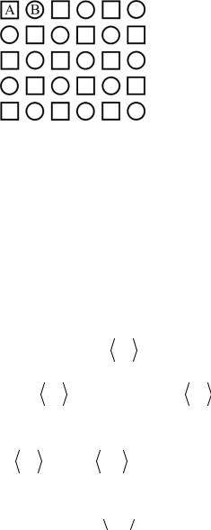
Fig. 28.2. Sublattices A and B with alternating arrangement of the nodes

Let us write the Hamiltonian considering the division on embedded sublattices. If the i-th magnetic moment refers to A-sublattice, we shall

denote it as iA . Analogously, if the i-th magnetic moment refers to B-

sublattice, we shall denote it as iB . We shall write σiA and σiB for pro-

jection operators of these magnetic moments for A- and B-sublattices, respectively. For example, the sum throughout the whole lattice consists of two sums for each sublattice

			(28.4)
∑σiz = ∑σiA z + ∑σiB z .			(28.4)
i	iA	iB

The Hamiltonian has the following form

						=
	H	= −∑σiz h + ∑Jij			σjz	=
		i		j≠i				(28.5)
		∑JiA j						(28.5)
= −∑σiA z h +		∑JiA j	σjz	−∑σiB z h + ∑JiB j σjz			.
iA		j≠iA		iB		j≠iB

Since we consider that only neighboring magnetic moments interact with each other then

		≡ zJxB ,	(28.6)
∑JiA j σjz	= ∑JiA jB σjB z	≡ zJxB ,	(28.6)
j≠iA	jB

where JiA jB = J for neighboring magnetic moments and z is the number of the nearest neighbors. Here we denote σjB z = xB : it is the mean value of magnetic moment projection in B-sublattice. We consider that

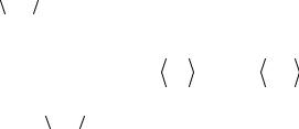
σjB z does not depend on the magnetic moment position in B-

sublattice, since all these moments are located in the same environment of magnetic moment from A-sublattice. Analogously

		≡ zJxA ,	(28.7)
∑JiB j σjz	= ∑JiB jA σjA z	≡ zJxA ,	(28.7)
j≠iB	jA

where σjA z = xA is the mean value of magnetic moment projection in

A-sublattice. Therefore we have two different order parameters: xA for A-sublattice and xB B-sublattice. Finally, for our Hamiltonian we obtain

			(28.8)
H	= −∑σiA z (h + zJxB )−∑σiB z (h + zJxA ).		(28.8)
	iA	iB

Denote the effective magnetic fields acting on A- and B-sublattices, respectively

hA = h + zJx ;

eff B

heffB = h + zJxA .

Therefore the Hamiltonian takes the following form

	A	B
H	= −heff ∑σiA z −heff ∑σiB z .
	iA	iB

(28.9)

(28.10)

As in the case of ferromagnets, we obtain the Hamiltonian of noninteracting magnetic moments placed into the “effective external field” dis-

tinct	for	each sublattice.		Denote	ˆ	A	and
tinct	for	each sublattice.		Denote	HA = −heff ∑σiA z		and
						iA
ˆ	B
HB = −heff ∑σiB z , and rewrite our Hamiltonian in the following form
		iB
		ˆ	ˆ	ˆ			(28.11)
		H = HA + HB .					(28.11)
	ˆ			ˆ
Since HA		acts only on A-sublattice and HB acts only on B-sublattice

)

−HA

xA ≡

Tr (σiA ze

heff

σiA z

= tanh

Tr (e

)

−HA

)

−HB

Tr (σiB ze

heff

xB ≡

σiB z

= tanh

Tr (e

)

−HB T

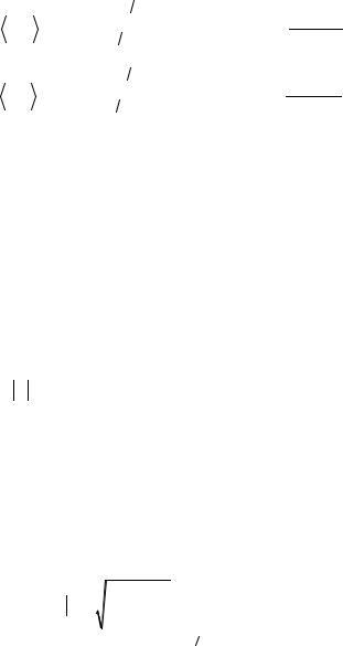
In the absence of magnetic field we obtain

= tanh

zJxB

;

zJxA

= tanh

tanh h + zJxB ;

tanh h + zJxA .

(28.12)

(28.13)

One can see that xA

and xB

have the different signs, since

us show that the solution with

xB = −xA

exists. Denote

xB = −x. Since J = −

< 0 we obtain

zJ (−x)

= tanh

Denote z J ≡TN , then

x= tanh x TN .

J < 0 . Let xA = x and

(28.14)

(28.15)

This equation has the same form as for a ferromagnet, but instead of Curie temperature θ one can see another temperature TN . The solution

is already known (see Fig. 28.3).

At T =TN the phase transition is take place, and order parameter be-

comes nonzero. All formulae that we obtained for ferromagnets (see § 14) are valid by replacing the Curie temperature θ on the TN

≈

−

, T →T

);

(28.16)

N−

≈1−2e−2TN T , T → 0.

(28.17)

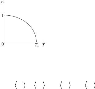
The value TN is called the Neél temperature or transition temperature into antiferromagnetic state.

Fig. 28.3. Parameter order dependence on temperature for antiferromagnets

Since xB = −x , at T =TN the spontaneous magnetization occurs in

every sublattice, but atomic magnetic moments in these sublattices are oppositely directed. Total magnetic moments of A- and B-sublattices are equal in magnitude and opposite in direction. That is why the total magnetization is equal to zero

µiA z

+ µiB z

µB

σiA z

+µB

σiB z

M =

(28.18)

+µ

−µ

B A 2

B B 2

= 0.

∂M

But the differential

magnetic

susceptibility

may not

χ =

∂H

H →0

equal to zero in contrast to χ =

M .

29. Magnetic susceptibility of the Ising antiferromagnet in the mean-field approximation

As we have seen, the total magnetization in antiferromagnet is equal

to zero. Therefore the magnetic susceptibility	χ =	M	is equal to zero as
		H

Источник: https://studfile.net/preview/16708691/

Смотрите также:

_1966(~1
"Логистическая технология JIT"
"Особенности правовой системы Российской Федерации" по дисциплине "Теория государства и права"
«Анализ ликвидности и платежеспособности предприятия» (на материалах ОАО Московская кондитерская фабрика «Красный Октябрь»)
«Дизайнерские дети» как профилактика инвалидизации общества
«ЗЕМЕЛЬНЫЕ РЕСУРСЫ КРАСНОДАРСКОГО КРАЯ»
«Методы учета затрат на производство продукции, работ, услуг»Курсовая работа
[2 курс] Определения
00438
00463