Материал: Маслов ИНТРОДУЦТИОН ТО ПХЫСИЦС ОФ СЕЦОНД-ОРДЕР МАГНЕТИЦ 2015
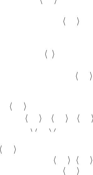
thermodynamic average  σ1z σ2 z
  T is called the correlation function. In
a crystal with regular atomic arrangement it depends on a relative position of two atoms:
|
|
|
|
(25.1) |
g(R1 |
− R2 ) = σ1z σ2z . |
|||
|
|
|
T |
|
In the mean field approximation we had |
|
|
||
|
|
0, T > θ; |
(25.2) |
|
g(R1 |
− R2 ) = |
, T < θ |
||
|
|
x2 |
|
|
|
is the order parameter, see § 11. |
|
||
for any R1 ≠ R2 , where x = σiz |
|
|||
|
T |
|
|
|
To begin with consider the case T > θ where we expect the qualitative modifications to the mean field approximation. Note that for a sys-
|
|
N |
tem of N magnetic moments the average σ1z σ2z T |
is taken over 2 |
|
configurations. In one half of those configurations the moment µ1 is
directed “up” (that is, the eigenvalue σ1z of the operator σ1z equals to +1), while in another half it is directed “down” (σ1z = –1), and hence the
|
can be represented as |
|
|
|
|
|
||||
average σ1z σ2z T |
|
|
|
|
|
|||||
|
|
|
|
1 |
|
|
1 |
|
, |
(25.3) |
|
σ1z σ2z |
T |
= |
2 |
σ1z σ2z + |
+ |
2 |
σ1z σ2z − |
||
where the symbols  ...
... + and
+ and  ...
... − stand for the thermodynamic averag-
es over 2N-1 configurations with the fixed values of σ1z = +1 and σ1z = –1 respectively. Since in zero magnetic field the Hamiltonian and the value
|
are invariant with the direction of the z axis (as z → –z, |
||||||
of σ1z σ2z T |
|||||||
σiz → –σiz for every i), we have |
|
|
|
|
− , that is |
||
σ1z σ2z |
+ |
= σ1z σ2z |
|||||
|
|
|
|
|
|
(25.4) |
|
|
g(R1 |
− R2 ) = σ1z σ2z . |
|
||||
|
|
|
|
|
+ |
|
|
By virtue of the fact that σ1z = +1 in all configurations involved, from Eq. (25.4) one has
66

|
|
|
|
|
|
|
|
|
|
Tr+ σ2z exp(−H / T ) |
|
|
|||||
g(R1 |
− R2 ) = |
σ2z + |
= |
|
|
|
, |
(25.5) |
|
|
/ T ) |
||||||
|
|
|
|
Tr+ exp(−H |
|
|
||
where the symbol Tr+ implies summation over the diagonal matrix elements calculated for the states with σ1z = +1 only.
Let us now rewrite the Hamiltonian of the Ising model, Eq. (10.7), separating out the terms that account for interactions of the magnetic moment µ2 with all other moments:
|
|
|
1 |
∑ |
/ |
|
(25.6) |
H |
= −∑J2 j σ2z σjz − |
|
|
Jij σiz σjz |
|||
|
j≠2 |
|
2 i, j≠2 |
|
|
|
|
(the external magnetic field H = 0). Next we apply the mean field approximation to the first part of Eq. (25.6), leaving the second one intact:
|
|
|
|
|
|
|
|
|
|
|
− |
|
H = −∑J2 j |
|
σ2z |
σjz |
+ σjz |
σ2z |
− σ2z |
σjz |
|
||||
j≠2 |
|
|
|
+ |
|
|
+ |
|
+ |
|
||
|
|
|
|
|
|
|
+ |
(25.7) |
||||
|
|
|
|
1 |
∑ |
/ |
|
|
|
|
|
|
|
|
|
− |
|
|
|
|
|
||||
|
|
|
|
|
Jij σiz σjz . |
|
|
|
|
|||
|
|
|
|
2 i, j≠2 |
|
|
|
|
|
|
|
|
In doing so, we neglect only the interactions between the fluctuations of the magnetic moment µ2 and fluctuations of other moments, while the
interactions between the fluctuations of all remaining moments are tak-
en |
into |
account without any approximations. Let us write |
|
(2) |
|
H |
= H |
+ ∆H , where |
|
(2) |
|
|
|
(25.8) |
|
H |
= −∑J2 j σjz |
σ2z |
||
|
|
j≠2 |
|
+ |
|
|
|
|
|
|
|
|
|
|
|
|
|
and ∆H |
is the rest of H . Considering that |
H does not contain the op- |
|||
|
|
|
in Eq. (25.5) we find |
|
|
erator σ2 z , for the average |
σ2z + |
|
|||
67
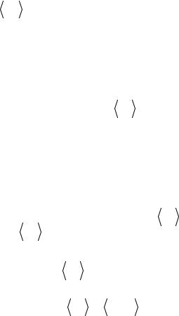
|
|
|
(2) |
|
|
|
|
|
|
|
|
Tr+ σ2z exp(−H |
|
/ T )Tr+ exp(−∆H / T ) |
|
||||
σ2z + |
= |
|
|
|
|
|
|
|
= |
|
(2) |
|
|
|
|
|
|||
|
|
Tr+ exp(−H |
/ T )Tr+ exp(−∆H / T ) |
(25.9) |
|||||
|
|
|
|
|
(2) |
/ T ) |
|
||
|
|
|
|
|
|||||
|
|
= |
Tr+ σ2z exp(−H |
|
|
||||
|
|
|
|
(2) |
/ T ) |
|
|||
|
|
|
|
|
|
||||
|
|
|
Tr+ exp(−H |
|
|||||
Designating
|
, |
(25.10) |
h′ = ∑J2 j σjz |
||
j≠2 |
+ |
|
|
|
(2)
we see that H can be viewed as the Hamiltonian of the single magnetic moment µ2 placed in an effective magnetic field H / = H / ez where H / =h′/ µB , see Eq. (25.10). By analogy with an isolated magnet-
ic moment in the field H = Hez , see § 4, we come up with the expression
|
|
|
|
|
|
|
|
|
|
|
|
|
|
|
|
h′ |
|
|
∑J2 j σjz |
|
|
|
|||
|
|
|
j≠2 |
+ |
|
|
||||||
|
|
σ2z = tanh |
|
|
= tanh |
|
|
. |
(25.11) |
|||
|
|
T |
|
T |
||||||||
|
|
+ |
|
|
|
|
|
|
|
|
||
|
|
|
|
|
|
|
|
|
|
|
|
|
Because |
the |
averages |
|
|
|
are |
taken |
over configurations |
with |
|||
σjz |
+ |
|
||||||||||
σ1z = +1, one has |
|
|
|
|
|
|
|
|
|
|
||
|
|
|
|
|
|
. |
|
(25.12) |
||||
|
|
|
σjz |
+ |
= σ1z σjz + |
|
||||||
Recalling |
the |
definition |
of the |
correlation |
function |
g(R1 − R2 ) , |
see |
|||||
Eq. (25.4), and taking into account Eqs. (25.5), (25.11) and (25.12), we arrive at the following expression:
|
|
|
1 |
|
|
|
|
|
|
|
g(R1 |
− R2 ) = tanh |
∑J (Rj − R2 )g(R1 |
− Rj ) . |
(25.13) |
||||||
|
||||||||||
|
|
T |
j≠2 |
|
|
|
|
|
||
68

Writing down similar expressions for g(R1 − Rj ) at j ≠ 2, we obtain a
set of N coupled equations for correlation functions g(R1 − Ri ) with
i = 2, 3, ..., N .
The system of nonlinear equations (25.13) has no exact analytical solution. Let us find an approximate expression for g(R1 − R2 ) in the case that the distance R1 − R2 between the magnetic moments greatly ex-
ceeds the interatomic spacing a. In this case, at least one of two strong inequalities, R1 − Rj >> a and Rj − R2 >> a , should hold for any j, so
that either g(R1 − Rj ) <<1 (because there is no long range magnetic or-
der at T > θ) or J (Rj − R2 ) is exponentially small (see § 8), or combina-
tion of both. As a consequence, the argument of hyperbolic tangent in the right-hand side of Eq. (25.13) is much less than unity, and one can restrict himself to the first term in a Taylor series tanh(z) = z + … :
|
|
1 |
|
|
|
|
|
|
|
g(R1 |
− R2 ) = |
|
|
∑J (Rj − R2 )g(R1 |
− Rj ) . |
(25.14) |
|||
T |
|||||||||
|
|
|
j≠2 |
|
|
|
|
||
Denoting R1 − R2 = R and Rj − R2 = R′, we have |
|
|
|||||||
|
|
1 |
|
|
|
|
|
|
|
|
g(R) = |
|
|
∑J (R′)g(R − R′) . |
(25.15) |
||||
|
T |
|
|||||||
|
|
|
R′≠0 |
|
|
|
|
||
It only remains for us to supplement Eq. (25.15) with a boundary condition at R = 0 . Since g(R = 0) =  σiz σiz
  T =1 for any T, one can approximately write
|
δ |
1 |
δ |
δ δ |
|
|
|
g(R) = |
|
∑J (R′)g(R − R′) + δRδ,0 |
, |
(25.16) |
|
|
T |
|||||
|
|
Rδ′≠0 |
|
|
|
|
where δδ |
= 1 and 0 at R = |
0 and R ≠ 0 respectively. |
|
|||
R,0 |
|
|
|
|
|
|
69

Expanding the functions g(R) and J (R) into the Fourier series,
|
1 |
|
|
|
|
|
|
|
|
g(R) = |
∑g |
(q)exp(iqR); |
|||||||
N |
|||||||||
|
|
q |
|
|
|
|
|
||
|
1 |
|
|
|
|
|
|
|
|
J (R) = |
∑J |
(q)exp(iqR), |
|||||||
N |
|||||||||
|
|
q |
|
|
|
|
|
||
from Eq.(25.16) we have |
|
|
|
1 |
|
|
|
|
|
|
|
|
|
|
|
||||
g(q) =1 |
+ |
|
|
J |
(q)g(q) , |
||||
T |
|
||||||||
|
|
|
|
|
|
|
|
||
whence it follows that at T > θ
g(q) = 1−β1J (q) ,
(25.17)
(25.18)
(25.19)
where β = 1/T. We also present without proof the expression for g(q) at T < θ:
g(qδ) = Nx2δδ |
+ |
1− x2 |
δ |
, |
(25.20) |
|
|||||
q,0 |
|
1−β(1− x2 )J (q) |
|
|
|
where x is the temperature dependent order parameter. One can see that at T → θ (that is, at x → 0) Eq. (25.20) transforms into Eq. (25.19).
With g(q) at hand, it |
is straightforward to calculate g(R) , see |
|||
Eq. (25.17). However first we should find |
J (q) . Since we are interested |
|||
mainly in behavior of g(R) |
|
>> a , |
|
|
at |
R |
the major contribution to the |
||
|
|
|
|
|
sum over q in Eq. (25.17) comes from the region of small q. Expanding
J (q) in powers of qR and restricting ourselves to quadratic terms we have
|
|
|
|
|
(−iqR)2 |
. (25.21) |
|
J (q) = ∑J (R)exp(−iqR) = ∑J (R) 1 |
−iqR + |
2 |
|
||||
R |
≠0 |
R≠0 |
|
|
|
|
|
Inasmuch as |
∑J (R) |
is, by definition, the Curie temperature θ (recall |
|||||
|
R≠0 |
|
|
|
|
|
|
that we set kB = 1), and the second term in Eq. (25.21) equals to zero from the symmetry considerations, we arrive at
70