Материал: Маслов ИНТРОДУЦТИОН ТО ПХЫСИЦС ОФ СЕЦОНД-ОРДЕР МАГНЕТИЦ 2015

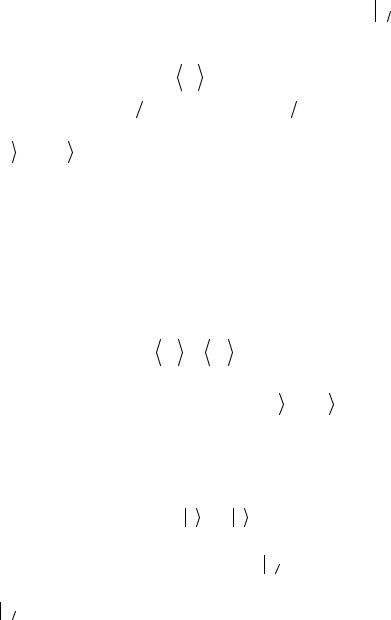
Внимание! Если размещение файла нарушает Ваши авторские права, то обязательно сообщите нам

At H > 0 the ground state (the state with the lowest energy) is ↑ with

µz = µ0.

Let us evaluate the value of µz at T ≠ 0:
µ	z	(T ) ≡ µ	z		= µ	P	−µ	P	,	(4.8)
	z		z	T	0	↑	0	↓
where P↑ = C exp(−E↑		T ) and		P↓ = C exp(−E↓					T )	are the statistical

(thermodynamic) probabilities to find the magnetic moment in the state

	↑ and	↓	respectively (hereafter the Boltzmann constant kB = 1).
	↑ and	↓	respectively (hereafter the Boltzmann constant kB = 1).
Calculating			the constant C from the				normalization	condition
	P↑ + P↓ =1, we have
			µz (T ) = µ0		µ	H		(4.9)
			µz (T ) = µ0	tanh	0		.	(4.9)
					T

In the limiting case T → 0 one has µz → µ0 at H > 0 (as shown above)

and µz → –µ0 at H < 0, while µz → 0 at T → ∞. At H = 0, the magnetic moment is zero regardless of T.

In the case that magnetic field is oriented along the z-axis, the magnetic moment projections on x and y axes are zero at any H and T:

			= 0 .	(4.10)
µx	T	= µy	= 0 .	(4.10)
	T		T

This is a consequence of zero values of quantum-mechanical averages

of the spin operators S x	and S y in the states		↑ and		↓ , see Eq. (1.8).

5. Interplay of quantum mechanics and statistics

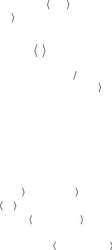
In order to calculate the temperature dependence of a physical quantity A, we first should solve the Schrödinger equation

	(5.1)
H n = En n ,

is the Hamiltonian of the system under consideration, and where H

find all eigenenergies En and eigenvectors n . Next we should work

out the quantum-mechanical averages of the operator in the states

n :

		An = n		n	(5.2)

			A
(note that the states	n

		need not be the eigenstates of A , that is,			A and

need not commute). Finally, the statistical (thermodynamic) average

is obtained as

A(T ) ≡				,		(5.3)
A(T ) ≡	A = ∑An Pn (T )			,		(5.3)
	T	n
where		n
where
Pn (T ) = C exp(−En T )						(5.4)
is the probability to find the system in the state					n	at temperature T.
is the probability to find the system in the state					n	at temperature T.
The constant C is determined from the condition ∑Pn (T ) =1 :
				n
C =		1	,			(5.5)
C =	∑exp(−En / T )		,			(5.5)
so that	n
so that	∑An exp(−En / T )
A(T ) =	∑An exp(−En / T )			.		(5.6)
	n
	∑exp(−En / T )

Let us derive a more general expression for A(T). It follows from Eq.

(5.1) that

n = exp(−En / T )

n . Therefore, with account

exp(−H / T )

for normalization n | n

=1, we have

∑exp(−En / T )= ∑ n

exp(−H / T )

≡Tr exp(−H / T ) (5.7)

and

∑An exp(

−En / T )

= ∑ n

n ≡

Aexp(−H / T )

(5.8)

≡Tr Aexp(−H / T )

so that


A(T ) =	Tr Aexp(−H / T )		.	(5.9)
		/ T )
	Tr exp(−H

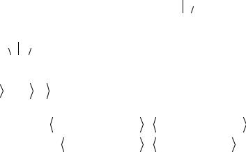
Since the trace (the sum of the diagonal matrix elements) of any operator does not depend on a specific set of states {n} used for its calcula-

tion, those states need not be the eigenstates of the Hamiltonian, they should just form the complete set and satisfy the orthonormality condi-

tion n m = δnm .The use of one or another set of states is a matter of

convenience. For example, in the case of isolated magnetic moment in an external magnetic field (§ 4), it is reasonable to choose

{

n }={

↑ ,

↓ }. Then

for

have from

A = µz

and H

= −µz H

Eq. (5.9):

H / T )

exp(

↑

↑ + ↓

↓

µz (T ) =

µz exp(µz

µz

µz H / T )

↑

exp(µz

H / T )

↑ + ↓

exp(µz H / T )

↓

(5.10)

exp(

H / T )−µ

exp(−µ

H / T )

= µ0

tanh

exp(µ0 H / T )+ exp(−µ0 H / T )

in accordance with Eq. (4.9).

6. A system of noninteracting local magnetic moments in an external magnetic field. Curie law

Having discussed the behavior of a single local magnetic moment in

an external magnetic field H , we now turn to a macroscopic system of N 1 local magnetic moments in a solid. Our purpose is to calculate

the experimentally measured magnetization M as a function of H and T.

Two types of interactions contribute to the total energy E of such a system: 1) the interaction of each magnetic moment with the magnetic field; 2) the interaction of the magnetic moments to one another, so that

N			(6.1)
E = ∑(−µi H )+Uint ({µi }),

i=1

and hence the Hamiltonian is

	N
				(6.2)
H	= −H ∑µi	+Uint ({µi }).
	i=1
Taking the z-axis along the magnetic field, H = Hez , we have
	N		}).
				(6.3)
H	= −H ∑µiz +Uint ({µi

i=1

In the case that magnetic moments weakly interact with one another (for example, because of their low concentration and/or small absolute values), one can neglect the term Uint in Eq. (6.3). Then the Hamiltonian of the whole system is just the sum of Hamiltonians of individual magnetic

moments, each being in the field H , and for the thermodynamic average of an arbitrary k-th magnetic moment we have

Trµk exp(−H / T )

µk (T ) =

Tr exp(−H / T )

k µk exp(

µk z H / T )Tr

i≠k exp ∑µi z H / T

i≠k

(6.4)

exp(µk z H

/ T )Tr

i≠k exp

∑µi z

H / T

i≠k

µk exp(

µk z H / T )

k exp(µk z H / T )Tr

i≠k

where Trk and Tri≠k stand for the trace over the states of, respectively,

k-th and all other magnetic moments.

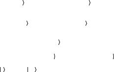
Let every magnetic moment in the system be associated with spin S =12 . Then the value of µkz(T) is given by Eq. (4.9) for an isolated

magnetic moment, while µkx(T) = µky(T) = 0, see § 4. Since all magnetic moments are identical, the total magnetic moment of the system is N

µk (T ) , and the magnetization equals to
	N
M (T, H ) =		µk (T )	= M (T, H )ez ,	(6.5)
	V

where

M (T, H ) = VN

In weak magnetic fields H << T/µ0 have from Eq. (6.6)

M (T, H )

µ0		µ	H		(6.6)
µ0	tanh	0		.	(6.6)
		T

(note that T/µ0 ~ 1 T at T = 1 K), we

≈	N	µ2	H	,	(6.7)
	V		T
		0

that is, M is linear in H, and the magnetic susceptibility χ = M/H equals to

χ(T ) =	N	µ2	1	.	(6.8)
	V
		0	T

Such temperature dependence of χ is referred to as Curie law. The fact that χ > 0 implies that materials containing noninteracting or weakly interacting magnetic moments are paramagnetic, see § 3.

7. Effective Weiss field

At H = 0 , magnetization M of a system of noninteracting local magnetic moments is zero at any temperature, see Eq. (6.6). Meanwhile,

there exist materials (ferromagnets) for which M ≠ 0 at H = 0 provid-

ed the temperature is below some characteristic value θ called the Curie temperature. It seems reasonable to assume that the failure to explane the occurrence of such materials within the model of noninteracting moments is a consequence of ignoring the interaction of magnetic moments with each other.

Weiss was the first who appreciated this. He noted that once the magnetic field H is applied to the sample, each moment µi interacts

not only with this field but with the field created by all other moments µk ≠i as well. Since, first, the magnetic field induced in the sample by an

external field H is

	4π N
4πM =		∑		(7.1)
	V		µk
		k =1		T

Источник: https://studfile.net/preview/16708691/

Смотрите также:

_1966(~1
"Логистическая технология JIT"
"Особенности правовой системы Российской Федерации" по дисциплине "Теория государства и права"
«Анализ ликвидности и платежеспособности предприятия» (на материалах ОАО Московская кондитерская фабрика «Красный Октябрь»)
«Дизайнерские дети» как профилактика инвалидизации общества
«ЗЕМЕЛЬНЫЕ РЕСУРСЫ КРАСНОДАРСКОГО КРАЯ»
«Методы учета затрат на производство продукции, работ, услуг»Курсовая работа
[2 курс] Определения
00438
00463