Материал: [2.1] 3D Imaging, Analysis and Applications-Springer-Verlag London (2012)

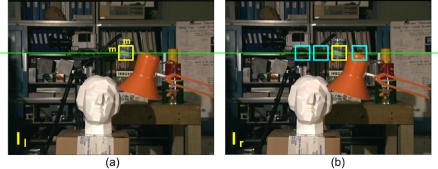
Fig. 2.11 Correlation-based methods look for the matching image window between the left and right rectified images. An m by m window centering at the pixel is used for correlation (Raw image pair courtesy of the Middlebury Stereo Vision Page [34], originally sourced from Tsukuba University)

The dissimilarity can be measured by the Sum of Squared Differences (SSD) cost for instance, which is the intensity difference as a function of disparity d :

where Il and Ir refer to the intensities of the left and right images respectively.

If two image windows correspond to the same world object, the pixel values of the windows should be similar and hence the SSD value would be relatively small. As shown in Fig. 2.11, for each pixel in the left image, correlation-based methods would compare the SSD measure for pixels within a search range along the corresponding epipolar line in the right image. The disparity value that gives the lowest SSD value indicates the best match.

A slight variation of SSD is the Sum of Absolute Differences (SAD) where the absolute values of the differences are added instead of the squared values:

This cost measure is less computationally expensive as it avoids the multiplication operation required for SSD. On the other hand, the SSD cost function penalizes the large intensity difference more due to the squaring operation.

The intensities between the two image windows may vary due to illumination changes and non-Lambertian reflection. Even if the two images are captured at the same time by two cameras with identical models, non-Lambertian reflection and differences in the gain and sensitivity can cause variation in the intensity. In these cases, SSD or SAD may not give a low value even for the correct matches. For these reasons, it is a good idea to normalize the pixels in each window. A first level of normalization would be to ensure that the intensities in each window are zeromean. A second level of normalization would be to scale the zero-mean intensities so that they either have the same range or, preferably, unit variance. This can be

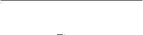
achieved by dividing each pixel intensity by the standard deviation of window pixel intensities, after the zero mean operation, i.e. normalized pixel intensities are given as:

While SSD measures the dissimilarity and hence the smaller the better, Normalized Cross-Correlation (NCC) measures the similarity and hence, the larger the better. Again, the pixel values in the image window are normalized first by subtracting the average intensity of the window so that only the relative variation would be correlated. The NCC measure is computed as follows:

2.7.2 Feature-Based Methods

Rather than matching each pixel, feature-based methods only search for correspondences to a sparse set of features, such as those located by a repeatable, welllocalized interest point detector (e.g. a corner detector). Apart from locating the features, feature extraction algorithms also compute some sort of feature descriptors for their representation, which can be used for the similarity criterion. The correct correspondence is given by the most similar feature pair, the one with the minimum distance between the feature descriptors.

Stable features are preferred in feature-based methods to facilitate matching between images. Typical examples of image features are edge points, lines and corners. For example, a feature descriptor for a line could contain the length, the orientation, coordinates of the midpoint or the average contrast along the edge line. A problem with linear features is that the matching can be poorly localized along the length of a line particularly if a linear feature is fragmented (imagine a smaller fragment from the left image sliding along a larger fragment from the right image). This is known as the aperture problem, referring to the fact that a local match ‘looks through’ a small aperture.

As a consequence, point-based features that are well-localized in two mutually orthogonal directions, have been preferred by researchers and practitioners in the field of computer vision. For example, the Harris corner detector [18] extracts points

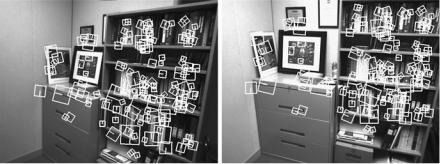
Fig. 2.12 Wide baseline matching between two images with SIFT. The size and orientation of the squares correspond to the scale and orientation of the matching SIFT features

that differ as much as possible from neighboring points. This is achieved by looking for high curvatures in two mutually orthogonal directions, as the gradient is illdefined in the neighborhood of corners. The corner strength or the grayscale values in a window region around each corner could be used as the descriptor. Another corner detector SUSAN [52] detects features based on the size, centroid and second moments of the local areas. As it does not compute image derivatives, it is robust to noise and does not require image smoothing.

Wide baseline matching refers to the situation where the two camera views differ considerably. Here, matching has to operate successfully over more difficult conditions, since there are larger geometric and photometric variations between the images.

In recent years, many interest point detection algorithms have been proposed that are scale invariant and viewpoint invariant to a certain extent which facilitates wide baseline matching. An interest point refers to an image feature that is stable under local and global perturbation and the local image structure is rich in terms of local image contents. These features are often described by a distinctive feature descriptor which is used as the similarity criterion. They can be used even when epipolar geometry is not yet known, as such distinctive descriptors allow correspondences to be searched over the whole image relatively efficiently.

For example, the Scale Invariant Feature Transform (SIFT) [28] and the SpeededUp Robust Feature (SURF) [2] are two popular features which were developed for image feature generation in object recognition applications. The SIFT feature is described by a local image vector with 128 elements, which is invariant to image translation, scaling, rotation and partially invariant to illumination changes and affine or 3D projections.

Figure 2.12 shows an example of matching SIFT features across large baseline and viewpoint variation. It can be seen that most matches are correct, thanks to the invariance and discriminative nature of SIFT features.

2.8 3D Reconstruction

Different types of 3D reconstruction can be obtained based on the amount of a priori knowledge available, as illustrated in Table 2.2. The simplest method to recover 3D information is stereo where the intrinsic and extrinsic parameters are known and the absolute metric 3D reconstruction can be obtained. This means we can determine the actual dimensions of structures, such as: height of door = 1.93 m.

For structure from motion, if no such prior information is available, only a projective 3D reconstruction can be obtained. This means that 3D structure is known only up to an arbitrary projective transformation so we know, for example, how many planar faces the object has and what point features are collinear, but we do not know anything about the scene dimensions and angular measurements within the scene. If intrinsic parameters are available, the projective 3D reconstruction can be upgraded to a metric reconstruction, where the 3D reconstruction is known up to a scale factor (i.e. a scaled version of the original scene). There is more detail to this hierarchy of reconstruction than we can present here (for example affine 3D reconstruction lies between the metric and projective reconstructions) and we refer the interested reader to [21].

2.8.1 Stereo

Stereo vision refers to the ability to infer information on the 3D structure and distance of a scene from two or more images taken from different viewpoints. The disparities of all the image points form the disparity map, which can be displayed as an image. If the stereo system is calibrated, the disparity map can be converted to a 3D point cloud representing the scene.

The discussion here focuses on binocular stereo for two image views only. Please refer to [51] for a survey of multiple-view stereo methods that reconstruct a complete 3D model instead of just a single disparity map, which generates range image information only. In such a 3D imaging scenario, there is at most one depth per image plane point, rear facing surfaces and other self-occlusions are not imaged and the data is sometimes referred to as 2.5D.

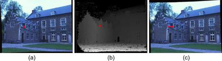
Fig. 2.13 A sample disparity map (b) obtained from the left image (a) and the right image (c). The disparity value for the pixel highlighted in red in the disparity map corresponds to the length of the line linking the matching features in the right image. Figure courtesy of [43]

2.8.1.1 Dense Stereo Matching

The aim of dense stereo matching is to compute disparity values for all the image points from which a dense 3D point cloud can be obtained. Correlation-based methods provide dense correspondences while feature-based methods only provide sparse correspondences. Dense stereo matching is more challenging than sparse correspondences as textureless regions do not provide information to distinguish the correct matches from the incorrect ones. The quality of correlation-based matching results depends highly on the amount of texture available in the images and the illumination conditions.

Figure 2.13 shows a sample disparity map after dense stereo matching. The disparity map is shown in the middle with disparity values encoded in grayscale level. The brighter pixels refer to larger disparities which mean the object is closer. For example, the ground pixels are brighter than the building pixels. An example of correspondences is highlighted in red in the figure. The pixel itself and the matching pixel are marked and linked on the right image. The length of the line corresponds to the disparity value highlighted in the disparity map.

Comparing image windows between two images could be ambiguous. Various matching constraints can be applied to help reduce the ambiguity, such as:

•Epipolar constraint

•Ordering constraint

•Uniqueness constraint

•Disparity range constraint

The epipolar constraint reduces the search from 2D to the epipolar line only, as has been described in Sect. 2.5. The ordering constraint means that if pixel b is to the right of a in the left image, then the correct correspondences a and b must also follow the same order (i.e. b is to the right of a in the right image). This constraint fails if there is occlusion.

The uniqueness constraint means that each pixel has at most one corresponding pixel. In general, there is a one-to-one correspondence for each pixel, but there is none in the case of occlusion or noisy pixels.