Материал: [2.1] 3D Imaging, Analysis and Applications-Springer-Verlag London (2012)

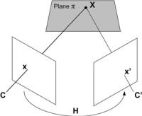
Fig. 2.9 The homography induced by a plane π , where a point x in the first image can be transferred to the point x in the second image

We can think of this homography as a mapping of image coordinates onto normalized coordinates (centered on the principal point at a unit metric distance from the camera). These points are rotated and then multiplying by K generates the image coordinates on the focal plane of the second, rotated camera.

2.5.6 Two Views of a Planar Scene

A homography should also be estimated for planar scenes where correspondences cannot uniquely define the epipolar geometry and hence the fundamental matrix. Similar to Eq. (2.7), the 2D-to-2D projection of the world plane π in Fig. 2.9 to the left and right images are given by:

λx x = Hx X, λx x = Hx X,

where Hx , Hx are 3 × 3 homography matrices (homographies) and x, x are homogeneous image coordinates. The planar homographies form a group and hence we can form a composite homography as H = Hx H−x 1 and it is straightforward to show that:

λx = Hx.

Figure 2.9 illustrates this mapping from x to x and we say that a homography is induced by the plane π . Homography estimation follows the same approach as was described in Sect. 2.4.1 for a scene-to-image planar homography (replacing X with x and x with x in Eqs. (2.8) to (2.10)).

Note that a minimum of four correspondences (no three points collinear in either image) are required because, for the homography, each correspondence generates a pair of constraints. Larger numbers of correspondences allow a least squares solution to an over-determined system of linear equations. Again suitable normalizations are required before SVD is applied to determine the homography.

A RANSAC-based technique can also be used to handle outliers, similar to the fundamental matrix estimation method described in Sect. 2.5.4. By repeatedly selecting the minimal set of four correspondences randomly to compute H and counting the number of inliers, the H with the largest number of inliers can be chosen.

Additional matches that are not in the original set of putative correspondences can be obtained using the best H. Then, H can be re-computed using all supporting matches in a linear least squares minimization using SVD.

Finally we note that, as in the case of the fundamental matrix, a non-linear optimization can be applied to refine the homography solution, if required by the application. The interested reader is referred to [21] for the details of the geometric cost function to be minimized.

2.6 Rectification

Typically, in a stereo rig, the cameras are horizontally displaced and rotated towards each other by an equal amount (verged), in order to overlap their fields of view. In this case, epipolar lines lie at a variety of angles across the two images, complicating the search for correspondences. In contrast, if these cameras had their principal axes parallel to each other (no vergence) and the two cameras had identical intrinsic parameters, conjugate (corresponding) epipolar lines would lie along the same horizontal scanline in each image, as observed in Sect. 2.5.3. This configuration is known as a standard rectilinear stereo rig. Clearly it is desirable to retain the improved stereo viewing volume associated with verged cameras and yet have the simplicity of correspondence search associated with a rectilinear rig.

To achieve this we can warp or rectify the raw images associated with the verged system such that corresponding epipolar lines become collinear and lie on the same scanline. A second advantage is that the equations for 3D reconstruction are very simply related to image disparity after image rectification, since they correspond to those of a simple rectilinear stereo rig. This triangulation computation is described later in the chapter.

Rectification can be achieved either with camera calibration information, for example in a typical stereo application, or without calibration information, for example in a typical structure from motion application. We discuss the calibrated case in the following subsection and give a brief mention of uncalibrated approaches in Sect. 2.6.2.

2.6.1 Rectification with Calibration Information

Here we assume a calibrated stereo rig, where we know both the intrinsic and the extrinsic parameters. Knowing this calibration information gives a simple rectification approach, where we find an image mapping that generates, from the original images, a pair of images that would have been obtained from a rectilinear rig. Of course, the field of view of each image is still bound by the real original cameras, and so the rectified images tend to be a different shape than the originals (e.g. slightly trapezoidal in a verged stereo rig).

Depending on the lenses used and the required accuracy of the application, it may be considered necessary to correct for radial distortion, using estimated parameters k1 and k2 from the calibration. To do the correction, we employ Eq. (2.6) in order to compute the unknown, undistorted pixel coordinates, [x, y]T , from the known distorted coordinates, [xd , yd ]T . Of course, an iterative solution is required for this non-linear equation and the undistorted pixel coordinates can be initialized to the distorted coordinates at the start of this process.

Assuming some vergence, we wish to map the image points onto a pair of (virtual) image planes that are parallel to the baseline and in the same plane. Thus we can use the homography structure in Eq. (2.19) that warps images between a pair of rotated views. Given that we already know the intrinsic camera parameters, we need to determine the rotation matrices associated with the rectification of the left and right views. We will assume that the origin of the stereo system is at the optical center of the left camera and calibration information gives [R, t] to define the rigid position of the right camera relative to this. To get the rotation matrix that we need to apply to image points of the left camera, we define the rectifying rotation matrix as:

rT1

Rrect = rT ,

2 rT3

where ri , i = 1 . . . 3 are a set of mutually orthogonal unit vectors. The first of these is in the direction of the epipole or, equivalently, the direction of the translation to the right camera, t. (This ensures that epipolar lines will be horizontal in the rectified image.) Hence the unit vector that we require is:

t r1 = t .

The second vector r2 is orthogonal to the first and obtained as the cross product of t and the original left optical axis [0, 0, 1]T followed by a normalization to unit length to give:

r2 = 1 [−ty , tx , 0]T . tx2 + ty2

The third vector is mutually orthogonal to the first two and so is computed using the cross product as r3 = r1 × r2.

Given that the real right camera is rotated relative to the real left camera, we need to apply a rotation RRrect to the image points of the right camera. Hence, applying homographies to left and right image points, using the form of Eq. (2.19), we have:

xrect = KRrectK−1x xrect = K RRrectK−1x ,

where K and K are the 3 × 3 matrices containing the intrinsic camera parameters for the left and right cameras respectively. Note that, even with the same make and

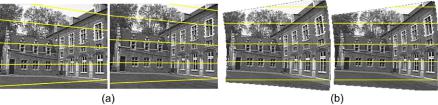
Fig. 2.10 An image pair before rectification (a) and after rectification (b). The overlay shows that the corresponding left and right features lie on the same image row after rectification. Figure courtesy of [43]

model of camera, we may find that the focal lengths associated with K and K are slightly different. Thus we need to scale one rectified image by the ratio of focal lengths in order to place them on the same focal plane.

As the rectified coordinates are, in general, not integer, resampling using some form of interpolation is required. The rectification is often implemented in reverse, so that the pixel values in the new image plane can be computed as a bilinear interpolation of the four closest pixels values in the old image plane. Rectified images give a very simple triangulation reconstruction procedure, which is described later in Sect. 2.8.1.2.

2.6.2 Rectification Without Calibration Information

When calibration information is not available, rectification can be achieved using an estimate of the fundamental matrix, which is computed from correspondences within the raw image data. A common approach is to compute a pair of rectifying homographies for the left and right images [20, 33] so that the fundamental matrix associated with the rectified images is the same form as that for a standard rectilinear rig and the ‘new cameras’ have the same intrinsic camera parameters. Since such rectifying homographies map the epipoles to infinity ([1, 0, 0]T ), this approach fails when the epipole lies within the image. This situation is common in structure from motion problems, when the camera translates in the direction of its Z-axis. Several authors have tackled this problem by directly resampling the original images along their epipolar lines, which are specified by an estimated fundamental matrix. For example, the image is reparameterized using polar coordinates around the epipoles to reduce the search ambiguity to half epipolar lines [42, 43]. Figure 2.10 shows an example of an image pair before and after rectification for this scheme, where the corresponding left and right features lie on the same image row afterwards. Specialized rectifications exist, for example [10] which allows image matching over large forward translations of the camera although, in this scheme, rotations are not catered for.

2.7 Finding Correspondences

Finding correspondences is an essential step for 3D reconstruction from multiple views. The correspondence problem can be viewed as a search problem, which asks, given a pixel in the left image, which is the corresponding pixel in the right image? Of course there is something of a circular dependency here. We need to find correspondences to determine the epipolar geometry, yet we need the epipolar geometry to find (denser) correspondences in an efficient manner. The RANSAC sampling approach described earlier, showed us how to break into this loop. Once we have the epipolar geometry constraint, the search space is reduced from a 2D search to the epipolar line only.

The following assumptions underpin most methods for finding correspondences in image pairs. These assumptions hold when the distance of the world point from the cameras is much larger than the baseline.

•Most scene points are visible from both viewpoints.

•Corresponding image regions are similar.

Two questions are involved: what is a suitable image element to match and what is a good similarity measure to adopt? There are two main classes of correspondence algorithms: correlation-based and feature-based methods. Correlation-based methods recover dense correspondences where the element to match is an image window centered on some pixel and the similarity measure is the correlation between the windows. Feature-based methods typically establish sparse correspondences where the element to match is an image feature and the similarity measure is the distance between descriptors of the image features.

2.7.1 Correlation-Based Methods

If the element to match is only a single image pixel, ambiguous matches exist. Therefore, windows are used for matching in correlation-based methods and the similarity criterion is a measure of the correlation between the two windows. A larger window gives larger image context which can reduce the probability of ambiguities, but this has its own problems which will be discussed in Sect. 2.8.1.1. The selected correspondence is given by the window that maximizes a similarity criterion or minimizes a dissimilarity criterion within a search range. Once a match is found, the offset between the two windows can be computed, which is called the disparity from which the depth can be recovered. Some commonly used criteria for correlation-based methods are described next.

Based on the rectified images in Fig. 2.11, we define the window function, where m, an odd integer, is the image window size so that: