Материал: [2.1] 3D Imaging, Analysis and Applications-Springer-Verlag London (2012)

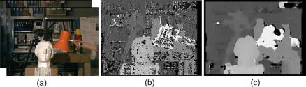
Fig. 2.14 The effect of window size on correlation-based methods: (a) input images (b) disparity map for a small correlation window (c) disparity map for a large correlation window (Raw image pair courtesy of the Middlebury Stereo Vision Page [34], originally sourced from Tsukuba University)

The disparity range constraint limits the disparity search range according to the prior information of the expected scene. Maximum disparity sets how close the object can be while the minimum disparity sets how far the object can be. Zero disparity refers to objects at infinity.

One important parameter for these correlation-based methods is the window size m in Eq. (2.20). While using a larger window size provides more intensity variation and hence more context for matching, this may cause problems around the occlusion area and at object boundaries, particularly for wide baseline matching.

Figure 2.14 shows the effect of window size on the resulting disparity map. The disparity map in the middle is for a window size of 3 × 3. It can be seen that, while it captures details well, it is very noisy, as the smaller window provides less information for matching. The disparity map on the right is for a window size of 15 × 15. It can be seen that while it looks very clean, the boundaries are not welldefined. Moreover, the use of a larger window size also increases the processing time as more pixels need to be correlated. The best window size is a trade-off between these two effects and is dependent on the level of fine detail in the scene.

For local methods, disparity computation at a given point depends on the intensity value within a local window only. The best matching window is indicated by the lowest dissimilarity measure or the highest similarity measure which uses information in the local region only. As pixels in an image are correlated (they may belong to the same object for instance), global methods could improve the stereo matching quality by making use of information outside the local window region.

Global methods perform optimization across the image and are often formulated as an energy minimization problem. Dynamic programming approaches [3, 5, 11] compute the minimum-cost path through the matrix of all pair-wise matching costs between two corresponding scanlines so that the best set of matches that satisfy the ordering constraint can be obtained. Dynamic programming utilizes information along each scanline independently, therefore, it may generate results that are not consistent across scanlines.

Graph cuts [6, 25] is one of the current state-of-the-art optimization techniques. These approaches make use of information across the whole image and produce high quality disparity maps. There is a trade-off between stereo matching quality

and the processing time. Global methods such as graph cuts, max flow [45], and belief propagation [53, 54] produce better disparity maps than local methods but they are very computationally intensive.

Apart from the algorithm itself, the processing time also depends on the image resolution, the window size and the disparity search range. The higher the image resolution, the more pixels need to be processed to produce the disparity map. The similarity measure needs to correlate more pixels for a larger window size. The disparity search range affects how many such measures need to be computed in order to find the correct match.

Hierarchical stereo matching methods have been proposed by down-sampling the original image into a pyramid [4, 44]. Dense stereo matching is first performed on the lowest resolution image and disparity ranges can be propagated back to the finer resolution image afterwards. This coarse-to-fine hierarchical approach allows fast computation to deal with a large disparity range, as a narrower disparity range can be used for the original image. Moreover, the more precise disparity search range helps to obtain better matches in the low texture areas.

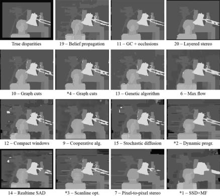
The Middlebury webpage [34] provides standard datasets with ground truth information for researchers to benchmark their algorithms so that the performance of various algorithms can be evaluated and compared. A wide spectrum of dense stereo matching algorithms have been benchmarked, as illustrated in Fig. 2.15 [46]. Researchers can submit results of new algorithms which are ranked based on various metrics, such as RMS error between computed disparity map and ground truth map, percentage of bad matching pixels and so on. It can be observed from Fig. 2.15 that it is very difficult to understand algorithmic performance by qualitative inspection of disparity maps and the quantitative measures presented in [46] are required.

2.8.1.2 Triangulation

When the corresponding left and right image points are known, two rays from the camera centers through the left and right image points can be back-projected. The two rays and the stereo baseline lie on a plane (the epipolar plane) and form a triangle, hence the reconstruction is termed ‘triangulation’. Here we describe triangulation for a rectilinear arrangement of two views or, equivalently, two rectified views.

After image rectification, the stereo geometry becomes quite simple as shown in Fig. 2.16, which shows the top-down view of a stereo system composed of two pinhole cameras. The necessary parameters, such as baseline and focal length, are obtained from the original stereo calibration. The following two equations can be obtained based on the geometry:

Fig. 2.15 Comparative disparity maps for the top fifteen dense stereo matching algorithms in [46] in decreasing order of performance. The top left disparity map is the ground truth. Performance here is measured as the percentage of bad matching pixels in regions where there are no occlusions. This varies from 1.15 % in algorithm 19 to 5.23 % in algorithm 1. Algorithms marked with a were implemented by the authors of [46], who present a wider range of algorithms in their publication. Figure courtesy of [46]

Fig. 2.16 The stereo geometry becomes quite simple after image rectification. The world coordinate frame is arbitrarily centered on the right camera. B is the stereo baseline and f is the focal length. Disparity is given by d = xc − xc

where xc and xc are the corresponding horizontal image coordinates (in metric units) in the right and left images respectively, f is the focal length and B is the baseline distance.

Disparity d is defined as the difference in horizontal image coordinates between the corresponding left and right image points, given by:

where yc is the vertical image coordinates in the right image.

This shows that the 3D world point can be computed once disparity is available: (xc , yc , d) → (X, Y, Z). Disparity maps can be converted into depth maps using these equations to generate a 3D point cloud. It can be seen that triangulation is straightforward compared to the earlier stages of computing the two-view relations and finding correspondences.

Stereo matches are found by seeking the minimum of some cost functions across the disparity search range. This computes a set of disparity estimates in some discretized space, typically integer disparities, which may not be accurate enough for 3D recovery. 3D reconstruction using such quantized disparity maps leads to many thin layers of the scene. Interpolation can be applied to obtain sub-pixel disparity accuracy, such as fitting a curve to the SSD values for the neighboring pixels to find the peak of the curve, which provides more accurate 3D world coordinates.

By taking the derivatives of Eq. (2.21), the standard deviation of depth is given by:

Z = Z2 d, Bf

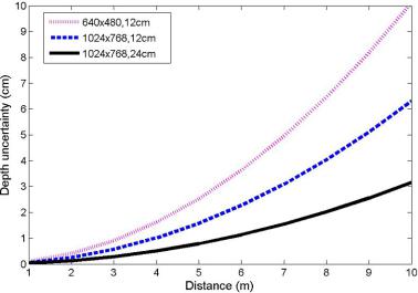
where d is the standard deviation of the disparity. This equation shows that the depth uncertainty increases quadratically with depth. Therefore, stereo systems typically are operated within a limited range. If the object is far away, the depth estimation becomes more uncertain. The depth error can be reduced by increasing the baseline, focal length or image resolution. However, each of these has detrimental effects. For example, increasing the baseline makes matching harder and causes viewed objects to self-occlude, increasing the focal length reduces the depth of field, and increasing image resolution increases processing time and data bandwidth requirements. Thus, we can see that design of stereo cameras typically involves a range of performance trade-offs, where trade-offs are selected according to the application requirements.

Figure 2.17 compares the depth uncertainty for three stereo configuration assuming a disparity standard deviation of 0.1 pixel. A stereo camera with higher

Fig. 2.17 A plot illustrating the stereo uncertainty with regard to image resolution and baseline distance. A larger baseline and higher resolution provide better accuracy, but each of these has other costs

resolution (dashed line) provides better accuracy than the one with lower resolution (dotted line). A stereo camera with a wider baseline (solid line) provides better accuracy than the one with a shorter baseline (dashed line).

A quick and simple method to evaluate the accuracy of 3D reconstruction, is to place a highly textured planar target at various depths from the sensor, fit a least squares plane to the measurements and measure the residual RMS error. In many cases, this gives us a good measure of depth repeatability, unless there are significant systematic errors, for example from inaccurate calibration of stereo camera parameters. In this case, more sophisticated processes and ground truth measurement equipment are required. Capturing images of a target of known size and shape at various depths, such as a textured cube, can indicate how reconstruction performs when measuring in all three spatial dimensions.

2.8.2 Structure from Motion

Structure from motion (SfM) is the simultaneous recovery of 3D structure and camera relative pose (position and orientation) from image correspondences and it refers to the situation where images are captured by a moving camera. There are three subproblems in structure from motion.

•Correspondence: which elements of an image frame correspond to which elements of the next frame.