Материал: [2.1] 3D Imaging, Analysis and Applications-Springer-Verlag London (2012)
3 Active 3D Imaging Systems |
99 |
which part of the projected pattern corresponds to which part of the imaged pattern.
When working with coherent light sources (lasers) eye-safety is of paramount importance and one should never operate laser-based 3D imaging sensors without appropriate eye-safety training. Many 3D imaging systems use a laser in the visible spectrum where fractions of a milliwatt are sufficient to cause eye damage, since the laser light density entering the pupil is magnified, at the retina, through the lens. For an operator using any laser, an important safety parameter is the maximum permissible exposure (MPE) which is defined as the level of laser radiation to which a person may be exposed without hazardous effect or adverse biological changes in the eye or skin [4]. The MPE varies with wavelength and operating conditions of a system. We do not have space to discuss eye safety extensively here and refer the reader to the American National Standard for Safe use of Lasers [4]. Note that high power low coherence (and non-coherent) light sources can also pose eye safety issues.
3.1.4 Chapter Outline
Firstly, we will present spot scanners and this will be followed by stripe scanners. Those types of scanners are used to introduce the concepts needed for the presentation of structured light systems in Sect. 3.4. In the following section, we discuss the calibration of active 3D imaging systems. Then, the measurement uncertainty associated with triangulation systems is presented. This section is optional advanced material and may be omitted on the first reading. The experimental characterization of active 3D imaging systems is then presented. In Sect. 3.8, further advanced topics are included and this section also may be omitted on the first reading. Towards the end of the chapter, we present the main challenges for future research, concluding remarks and suggestions for further reading. Finally a set of questions and exercises are presented for the reader to develop and consolidate their understanding of active 3D imaging systems.
3.2 Spot Scanners
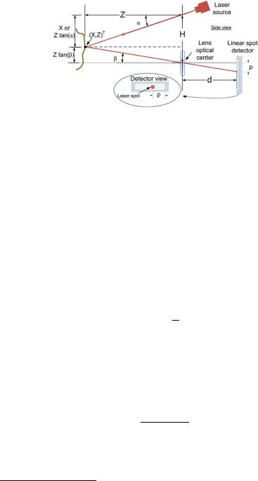
Usually, spot scanners use a laser. We limit the discussion to this type of technology and in order to study the basic principle of triangulation, we assume an infinitely thin laser beam diameter and constrain the problem to the plane (X, Z), i.e. Y = 0. The basic geometrical principle of optical triangulation for a spot scanner is shown in Fig. 3.2 and is identical to the one of passive stereo discussed in Chap. 2.
In Fig. 3.2, a laser source projects a beam of light on a surface of interest. The light scattered by that surface is collected from a vantage point spatially distinct from the projected light beam. This light is focused (imaged) onto a linear spot
100 |
M.-A. Drouin and J.-A. Beraldin |
Fig. 3.2 Schematic diagram of a single point optical triangulation sensor based on a laser beam and a linear spot detector. The baseline is H and d is the distance between the lens and the linear spot detector. The projection angle is α. The collection angle is β and it is computed using the distance d and the position p on the linear spot detector. The point [X, Z]T is determined by the baseline H , the projection angle α and the collection angle β. Figure courtesy of [11]
detector.1 The knowledge of both projection and collection angles (α and β) relative to a baseline (H ) determines the [X, Z]T coordinate of a point on a surface. Note that it is assumed that the only light that traverses the lens goes through the optical center, which is the well-known pinhole model of the imaging process. Furthermore, we refer to projection of the laser light onto the scene and we can think of the imaged spot position on the detector and the lens optical center as a back-projected ray, traveling in the opposite direction to the light, back into the scene. This intersects with the projected laser ray to determine the 3D scene point.
The linear spot detector acts as an angle sensor and provides signals that are interpreted as a position p. Explicitly, given the value of p, the value of β in radians is computed as
p |
|
|
β = arctan d |
(3.1) |
where d is the distance between the laser spot detector and the collection lens. (Typically this distance will be slightly larger than the focal length of the lens, such that the imaged spot is well focused at the depth at which most parts of the object surface are imaged. The relevant thin lens equation is discussed in Sect. 3.8.1.)
The position of p on the linear spot detector is computed using a peak detector which will be described later. Using simple trigonometry, one can verify that
H
Z = (3.2) tan α + tan β
and
X = Z tan α. |
(3.3) |
1A linear spot detector can be conceptually viewed as a conventional camera that has a singe row of pixels. Many linear spot detectors have been proposed in the past for 3D imaging [11].

3 Active 3D Imaging Systems |
|
|
|
101 |
|
Substituting Eq. (3.1) into Eq. (3.2) gives |
|
|
|
||
Z = |
|
H d |
(3.4) |
||
|
|
|
. |
||
p |
+ |
d tan α |
|||
|
|
|
|
|
|
In order to acquire a complete profile without using a translation stage, the laser beam can be scanned around some [X, Z]T coordinate using a mirror mounted on a mechanical scanner (typically a galvonometer drive). In this case, the angle α is varied according to a predefined field of view. For practical reasons, the total scanned angle for a configuration like the one in Fig. 3.2 is about 30 degrees. Larger angles may be scanned by more sophisticated optical arrangements called synchronized scanners, where the field of view of the camera is scanned using the same mirror that scans the laser. Sometimes the reverse side of a double sided mirror is used [21, 54].
3.2.1 Spot Position Detection
It is crucial to obtain the position of the laser spot on the linear spot detector to sub-pixel accuracy. In order to accomplish this, the image of the laser spot must be a few pixels wide on the detector which is easy to achieve in a real system. Many peak detectors have been proposed to compute the position of the laser spot and two studies compare different peak detectors [34, 48]. We examine two peak detectors [18, 34, 48]. The first one localizes the ‘center of mass’ of the imaged spot intensity. In this method, the pixel iM with the maximum intensity is found in the 1D image which is denoted I . Then a window of size 2N + 1 centered on iM is used to compute the centroid position. Explicitly, the peak position p is defined as
|
= |
M + |
N |
I (iM + i)i |
|
|
|
N |
|
|
|||
p |
i |
|
i=−N |
. |
(3.5) |
|
|
|
|
i=−N I (iM + i) |
|
||
The second peak detector uses convolution with a derivative filter, followed by a linear interpolation. Explicitly, for each pixel, i, let
|
N |
|
j |
|
(3.6) |
g(i) = |
I (i − j )F (j + N ) |
=−N
where F = [1, 1, 1, 1, 0, −1, −1, −1, −1] and N = 4. Finally, the linear interpolation process is implemented as
g(i0) |
|
p = i0 + g(i0) − g(i0 + 1) |
(3.7) |
where i0 is a pixel such that g(i0) ≥ 0 and g(i0 + 1) < 0. Moreover, F has the property of filtering out some of the frequency content of the image [18]. This makes it
102 |
M.-A. Drouin and J.-A. Beraldin |
possible to filter out the ambient illumination and some of the noise and interference introduced by the linear detector electronics. Note that other filters could be used. It has been shown that the second peak detector outperforms the first in an actual implementation of laser triangulation [18].
3.3 Stripe Scanners
As shown previously, spot scanners intersect a detection direction (a line in a plane, which is a back-projected ray) with a projection direction (another line in the same plane) to compute a point in a 2D scene space. Stripe scanners and structured light systems intersect a back-projected 3D ray, generated from a pixel in a conventional camera, and a projected 3D plane of light, in order to compute a point in the 3D scene. Clearly, the scanner baseline should not be contained within the projected plane, otherwise we would not be able to detect the deformation of the stripe. (In this case, the imaged stripe lies along an epipolar line in the scanner camera.)
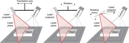
A stripe scanner is composed of a camera and a laser ‘sheet-of-light’ or plane, which is rotated or translated in order to scan the scene. (Of course, the object may be rotated on a turntable instead, or translated, and this is a common set up for industrial 3D scanning of objects on conveyer belts.) Figure 3.3 illustrates three types of stripe scanners. Note that other configurations exist, but are not described here [16]. In the remainder of this chapter, we will discuss systems in which only the plane of projected light is rotated and an image is acquired for each laser plane orientation. The camera pixels that view the intersection of the laser plane with the scene can be transformed into observation directions (see Fig. 3.3). Depending on the roll orientation of the camera with respect to the laser plane, the observation directions in the camera are obtained by applying a peak detector on each row or column of the camera image. We assume a configuration where a measurement is performed on each row of the camera image using a peak detector.
Next, the pinhole camera model presented in the previous chapter is revisited. Then, a laser-plane-projector model is presented. Finally, triangulation for a stripe scanner is described.
Fig. 3.3 (Left) A stripe scanner where the scanner head is translated. (Middle) A stripe scanner where the scanner head is rotated. (Right) A stripe scanner where a mirror rotates the laser beam. Figure courtesy of the National Research Council (NRC), Canada
3 Active 3D Imaging Systems |
103 |
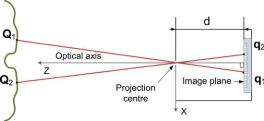
Fig. 3.4 Cross-section of a pinhole camera. The 3D points Q1 and Q2 are projected into the image plane as points q1 and q2 respectively. Finally, d is the distance between the image plane and the projection center. Figure courtesy of NRC Canada
3.3.1 Camera Model
The simplest mathematical model that can be used to represent a camera is the pinhole model. A pinhole camera can be assembled using a box in which a small hole (i.e. the aperture) is made on one side and a sheet of photosensitive paper is placed on the opposite side. Figure 3.4 is an illustration of a pinhole camera. The pinhole camera has a very small aperture so it requires long integration times; thus, machine vision applications use cameras with lenses which collect more light and hence require shorter integration times. Nevertheless, for many applications, the pinhole model is a valid approximation of a camera. In this mathematical model, the aperture and the photo-sensitive surface of the pinhole are represented respectively by the center of projection and the image plane. The center of projection is the origin of the camera coordinate system and the optical axis coincides with the Z-axis of the camera. Moreover, the optical axis is perpendicular to the image plane and the intersection of the optical axis and the image plane is the principal point (image center). Note that when approximating a camera with the pinhole model, the geometric distortions of the image introduced by the optical components of an actual camera are not taken into account. Geometric distortions will be discussed in Sect. 3.5. Other limitations of this model are described in Sect. 3.8.
A 3D point [Xc , Yc , Zc ]T in the camera reference frame can be transformed into pixel coordinates [x, y]T by first projecting [Xc , Yc , Zc ]T onto the normalized camera frame using [x , y ]T = [Xc /Zc , Yc /Zc ]T . This normalized frame corresponds to the 3D point being projected onto a conceptual imaging plane at a distance of one unit from the camera center. The pixel coordinates can be obtained from the normalized coordinates as
|
|
|
x |
|
|
|
|
|
y |
= |
d |
y |
|
+ |
|
x |
(3.8) |
|
sx |
oy |
|
|||||
x |
|
|
|
o |
|
|
||
sy
where sx and sy are the dimensions of the sensor in millimeters divided by the number of pixels along the X and Y -axis respectively. Moreover, d is the distance in millimeters between the aperture and the sensor chip and [ox , oy ]T is the position