Материал: [2.1] 3D Imaging, Analysis and Applications-Springer-Verlag London (2012)
3 Active 3D Imaging Systems |
109 |
possible to compute either the centers of the fringes or the edges between adjacent fringes in order to define the projector plane with which triangulation is performed. Generally edge based schemes give better performance [57].
3.4.1.1 Decoding of Binary Fringe-Based Codes
Two algorithms for transforming the camera images into correspondences between projector fringes and camera pixels are presented. In the first algorithm, the camera pixels are at known positions and the projector fringe for those positions are measured. In the second algorithm, the fringe indices are known in the projector and for each row of the camera the fringe transitions are measured.
The first algorithm uses a simple thresholding approach where a threshold is computed individually for each pixel of the camera [57]. The threshold values are computed using the images of the projection of a white and a black frame. For every camera pixel, the mean value of the white and black frames is used as the threshold value. This method does not allow a sub-pixel localization of the boundary between fringes, which is important in order to increase the precision of the system (see Sect. 3.6). This method simply classifies the camera pixel as being lit by which projector pixel and supports other coding strategies such as phase measurement methods covered in Sect. 3.4.2.
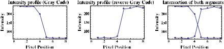
The second algorithm provides a robust way for achieving sub-pixel accuracy [63]. The method requires the projection of both a Gray code and the associated reverse Gray code (white fringes are replaced by black ones and vice versa). Figure 3.7 illustrates the process of computing the position of a stripe’s transition into the camera image. An intensity profile is constructed using linear interpolation for both the images of a Gray code and those of the associated reverse Gray code (left side and middle of Fig. 3.7). The intersection of both profiles is the sub-pixel location of the fringe transition (right side of Fig. 3.7).
Fig. 3.7 (Left) Intensity profile of a white-to-black transition in the image of a Gray code. The values between pixels are obtained using linear interpolation. The transition is located between the 4th and 5th pixel. (Middle) The same intensity profile for the associated reverse Gray code. (Right) The two previous graphs are superimposed and the intersection is marked with a dot. The transition is localized at pixel 4.45. Figure courtesy of NRC Canada
110 |
M.-A. Drouin and J.-A. Beraldin |
3.4.1.2 Advantage of the Gray Code
The Gray code offers a significant advantage over the natural binary code when using the previously described thresholding algorithm with noisy images. The reason for this is that more decoding errors occur on fringe transitions, namely pixels where the pattern changes from dark to light or light to dark. For the Gray code, there are significantly fewer fringe transitions over the N patterns when compared to the natural binary code. In fact the natural binary code has the highest possible frequency of transitions in the N th projected pattern, which corresponds to the least significant bit of the code.
Let us assume that the probability of getting an error when thresholding a camera image at a pixel located at a fringe transition is p, and that the probability of getting an error when no transition occurs is q, the probability of getting an error using a Gray code is p × qN −1 for all camera pixels located at a transition independent of the transition location. In this case, the Gray code results in a uniform distribution of error at the transition which is not the case with the natural binary code. The natural binary code has a probability of getting an error at a transition that ranges from pN to p × qN −1. As an example, the probability of getting an error at the transition between 7 and 8 and between 0 and 1 in the natural binary code shown in Table 3.1 are p4 (all bits change) and p × q3 respectively (only one bit changes). As we have already mentioned, in a fringe projection system, it is expected that p is larger than q. Thus, the mean error rate at fringe transitions when using a Gray code is expected to be smaller than the one obtained using a natural binary code.
The narrowest fringes of a Gray code may be difficult to decode and are errorprone when the images are out-of-focus (see Sect. 3.8). For this reason, a Gray code is often used to establish a coarse correspondence using the widest patterns and another code based on phase measurement replaces the narrowest patterns. Phase measurement methods (also known as phase shift) outperform Gray code methods when the patterns are out-of-focus. Phase shift methods are presented next.
3.4.2 Phase Shift Methods
While a Gray code is binary in nature (through a suitable thresholding of intensity images), phase shift approaches use patterns containing periodic and smooth variations in greyscale level. The phase shift patterns contain vertical fringes and each projector column, x2, is associated with a phase value φ (x2) using
φ (x2) = |
2π |
mod (x2, ω) |
(3.16) |
ω |
|||
where ω is the spatial period of the pattern and mod |
is the modulo operator. |
||
The intensity profile for each row is defined by I (x2) = A + B cos(φ (x2) − θ ) where A and B are constants and θ is a phase offset. Many patterns with different
3 Active 3D Imaging Systems |
111 |
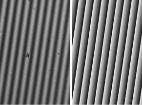
Fig. 3.8 (Left) the camera image of a phase shift pattern. (Right) the recovered phase for each camera pixel coded in greyscale level. The image is of the surface defect shown in Fig. 3.6(Left). Figure courtesy of NRC Canada
phase offset, θ , are required to establish the correspondence between the phase measured at a camera pixel and the phase associated with a projector fringe. Note that, because the modulo operator is used, this mapping is not unique and an extra unwrapping step is necessary to establish an unambiguous correspondence. Figure 3.8 shows a phase shift pattern and the recovered phase.
The intensity of each pixel of the camera viewing the projected phase shift patterns can be modeled using the following system of equations:
I0(x1, y1) = A(x1, y1) + B(x1, y1) cos φ (x1, y1) − θ0
I1(x1, y1) = A(x1, y1) + B(x1, y1) cos φ (x1, y1) − θ1
(3.17)
. . .
IN −1(x1, y1) = A(x1, y1) + B(x1, y1) cos φ (x1, y1) − θN −1
where A(x1, y1), B(x1, y1) and φ (x1, y1) are unknowns and θi are the known phase offsets in the projector. The number of patterns is N . Ii (x1, y1) is the measured image intensity for camera pixel [x1, y1]T when the pattern with the phase offset θi is projected. Using the trigonometric identity cos(α − β) = cos α cos β + sin α sin β, the previous system of equations is equivalent to
I0(x1, y1) = A(x1, y1) + B1(x1, y1) cos(θ0) + B2(x1, y1) sin(θ0)
I1(x1, y1) = A(x1, y1) + B1(x1, y1) cos(θ1) + B2(x1, y1) sin(θ1)
(3.18)
. . .
IN (x1, y1) = A(x1, y1) + B1(x1, y1) cos(θN −1) + B2(x1, y1) sin(θN −1)
where
B1(x1, y1) = B(x1, y1) cos φ (x1, y1) |
(3.19) |

112 |
|
|
|
|
|
M.-A. Drouin and J.-A. Beraldin |
|
and |
|
|
|
|
|
|
|
B2(x1, y1) = B(x1, y1) sin φ (x1, y1) . |
(3.20) |
||||||
Since the θi are known, cos θi |
and sin θi are scalar coefficients. The following more |
||||||
compact matrix notation can be used |
|
|
|
||||
|
|
MX(x1, y1) = I(x1, y1) |
|
(3.21) |
|||
where I(x1, y1) = [I0(x1, y1), I1(x1, y1), . . . , IN −1(x1, y1)]T , |
|
||||||
|
|
|
1 |
cos(θ1) |
sin(θ1) |
|
|
|
= |
|
1 cos(θ0) |
sin(θ0) |
|
|
|
M |
. |
. |
. |
(3.22) |
|||
|
|
|
. |
. |
. |
|
|
|
|
|
|
|
|
|
|
|
|
|
|
|
|
|
|
1 cos(θN −1) sin(θN −1)
and X(x1, y1) = [A(x1, y1), B1(x1, y1), B2(x1, y1)]T . In the presence of noise and when using more than three patterns, the system of equations may have no solution. In this case, the vector X(x1, y1) is obtained using the pseudoinverse and explicitly,
X(x1, y1) = MT M −1MT I(x1, y1). |
(3.23) |
Note that MT M is invertible when M has rank 3. Alternative presentations can be found in [31, 51]. Once X(x1, y1) is computed,
B(x1, y1) = |
B1(x1, y1)2 + B2(x1, y1)2 |
|
(3.24) |
and |
|
||
φ (x1, y1) = arctan B2(x1, y1), B1(x1, y1) |
(3.25) |
||
where arctan(n, d) represents the usual arctan(n/d) where the sign of n and d are used to determinate the quadrant.
We provide the details for the case θi = 2Nπ i for which |
|
|
|
|
|
|
|
|
||||||||||||||||
|
|
|
N 0 0 |
|
|
|
|
|
|
|
|
|
|
|
|
N −1 Ii (x1, y1) |
|
|
||||||
T |
|
|
N |
|
|
|
T |
|
|
N |
|
|
1 |
i=0 |
|
|
2iπ |
|||||||
M M |
= |
|
0 |
2 |
0 |
|
and M I(x1 |
, y1) |
= |
|
i |
|
− |
|
I |
(x |
, y |
) cos( |
N |
) . |
||||
|
|
|
|
|
|
|
|
|
|
|
0 |
i |
1 |
1 |
|
|
||||||||
|
|
|
|
|
|
|
|
|
|
|
= |
|
|
|
|
|
|
|
||||||
|
|
0 0 |
N |
|
|
|
|
|
N |
|
|
1 |
Ii (x1, y1) sin( |
2iπ |
||||||||||
|
|
|
|
|
2 |
|
|
|
|
|
|
|
i |
|
−0 |
N |
) |
|||||||
|
|
|
|
|
|
|
|
|
|
|
|
|
|
= |
|
|
|
|
|
|
|
|
||
Explicitly, A(x1, y1), B1(x1, y1) and B2(x1, y1) are computed using |
|
|
|
|||||||||||||||||||||
|
|
|
|
|
|
|
1 |
N −1 |
|
|
|
|
|
|
|
|
|
|
|
|
|
|
|
|
|
|
|
|
|
A(x1, y1) = |
|
Ii (x1, y1) |
|
|
|
|
|
|
|
|
|
|
|
(3.26) |
|||||
|
|
|
|
|
N |
|
|
|
|
|
|
|
|
|
|
|
||||||||
|
|
|
|
|
|
|
|
|
i=0 |
|
|
|
|
|
|
|
|
|
|
|
|
|
|
|
|
|
|
|
|
|
|
2 |
N −1 |
|
|
|
|
|
|
2iπ |
|
|
|
|
|
||||
|
|
|
|
|
B1(x1, y1) = |
|
Ii (x1, y1) cos |
|
|
|
|
|
(3.27) |
|||||||||||
|
|
|
|
|
N |
N |
|
|
|
|||||||||||||||
|
|
|
|
|
|
|
|
|
i=0 |
|
|
|
|
|
|
|
|
|
|
|
|
|
|
|

3 Active 3D Imaging Systems |
113 |
2 |
N −1 |
2iπ |
|
|
|
B2(x1, y1) = |
|
Ii (x1, y1) sin |
|
|
(3.28) |
N |
N |
||||
|
|
i=0 |
|
|
|
and φ (x1, y1) and B(x1, y1) are computed using Eq. (3.25) and Eq. (3.24) respectively.
3.4.2.1 Removing the Phase Ambiguity
Once the phases have been computed, projector position x2 corresponding to the camera pixel [x1, y1]T is given as
x2 = |
ω |
|
2π φ (x1, y1) + k(x1, y1) |
(3.29) |
where k(x1, y1) is an unknown integer that represents the phase ambiguity. The value of k(x1, y1) must be recovered in order to compute the location of the 3D points. We will briefly describe two different approaches that allow the removal of this phase ambiguity.
Fiducial markers can be embedded into the phase shift patterns. Those markers can simply be a white or black point. When there is only one marker, the 3D position of the surface on which the fiducial maker is projected can be computed by triangulation. This allows one to know the k values for the camera pixels around a fiducial marker. It is then possible to propagate this information to neighboring pixels using a phase unwrapping algorithm. Phase unwrapping is frequently encountered in other fields such as synthetic aperture radar and interferometry. This is a complex subject and an entire book is devoted to it [37]. For these reasons, phase unwrapping will not be discussed further. When the projection patterns contain many fiducial markers, the epipolar constraint and the ordering constraint which are described in the previous chapter can be used to establish unambiguous matches between fiducial markers. Note that a similar fiducial approach is implemented in [42].
The second approach combines phase shift and Gray codes [58]. Binary codes, such as the Gray code, are often used to establish a coarse correspondence between projector and camera pixels using the thresholding algorithm presented previously. The patterns with the smallest stripes are not projected and are replaced by phase shift patterns whose spatial periods are selected to match the smallest stripes projected. Combining binary and phase shift code is a solution used in many experimental [57] and commercial scanners.
3.4.3 Triangulation for a Structured Light System
In the projective-geometry framework of the pinhole camera, a digital projector can be viewed as an inverse camera and both share the same parametrization. Each implementation of an analogue slide projector can have its own parametrization.