Материал: [2.1] 3D Imaging, Analysis and Applications-Springer-Verlag London (2012)
104 M.-A. Drouin and J.-A. Beraldin
in pixels of the principal point (image center) in the image. The parameters sx , sy , d, ox and oy are the intrinsic parameters of the camera. Note that the camera model used in this chapter is similar to the one used in the previous chapter, with one minor difference: f mx and f my are replaced by d/sx and d/sy respectively. This change
1 |
1 |
|
||
is partly notational (mx = |
|
, my = |
|
) and partly to do with where the image is in |
sx |
sy |
|||
focus relative to the camera center (in general, d and f are not equal, with d often being slightly larger). This will be discussed further in Sect. 3.8. Note that intrinsic camera parameters can be determined using the method described in Chap. 2.
The extrinsic parameters of the camera must be defined in order to locate the position and orientation of the camera in the world coordinate system. This requires three parameters for the rotation and three parameters for the translation. (Note that in many design situations, we can define the world coordinate system such that it coincides with the camera coordinate system. However, we still would need to estimate the pose of the light projection system, which can be viewed as an inverse camera, within this frame. Also, many active 3D imaging systems use multiple cameras, which can reduce the area of the ‘missing parts’ caused by self occlusion.)
The rotation is represented using a 3 × 3 rotation matrix |
|
|
0 |
|||||||||
Rc |
0 |
cos θx |
− sin θx |
|
0 |
1 |
0 |
sin θz |
cos θz |
|||
|
1 |
0 |
0 |
|
cos θy |
0 |
sin θy |
|
cos |
θz |
− sin θz |
0 |
|
= 0 |
sin θx |
cos θx |
− sin θy |
0 |
cos θy |
|
0 |
|
0 |
1 |
|
(3.9)
where θx , θy and θz are the rotation angles around the X, Y , and Z axis and translation is represented by a vector Tc = [Tx , Ty , Tz]T . Note that the rotation matrix Rc
c |
= |
c |
T |
|
= |
1. |
|
is orthogonal (i.e. RT |
|
R−1) and det(R) |
|
|
|||
A 3D point Qw = [Xw , Yw , Zw ] |
Tin the world reference frame can be trans- |
||||||
formed into a point Qc = [Xc , Yc , Zc ] |
of the camera reference frame by using |
||||||
|
|
|
Qc = Rc Qw + Tc . |
(3.10) |
|||
Then, the point Qc is projected onto the normalized camera frame [x , y ]T =
Xc /Zc , Yc /Zc T . Finally, the point in the normalized camera frame x |
, y |
] |
T |
can be |
|||||||||||||||
[ |
] |
|
|
|
|
|
|
|
x, y |
T |
|
|
|
|
[ |
|
|
|
|
transformed into the pixel coordinate |
] using Eq. (3.8). Explicitly, the trans- |
||||||||||||||||||
formation from Qw to pixel [x, y]T is [ |
|
||||||||||||||||||
|
|
|
|
d (r11,r12,r13)Qw |
Tx |
|
|
|
|
|
|
|
|||||||
|
x |
= |
|
|
(r31,r32,r33)Qw |
++Tz |
|
ox |
|
|
|
|
|
||||||
|
sx |
|
|
|
(3.11) |
||||||||||||||
|
y |
|
d (r21,r22,r23)Qw +Ty |
|
+ oy |
|
|
|
|
||||||||||
|
|
|
sy |
|
(r31,r32,r33)Qw +Tz |
|
|
|
|
|
|
||||||||
where the rij |
are the elements of matrix Rc . Note that a pixel [x, y]T |
can be trans- |
|||||||||||||||||
formed into the normalized camera frame using |
|
|
|
|
|
|
|
||||||||||||
|
|
|
x |
1 |
|
sx (x |
|
ox ) |
|
|
|
|
|
(3.12) |
|||||
|
|
y |
= d |
sy (y |
− oy ) . |
|
|
|
|
||||||||||
|
|
|
|
|
|
|
|
|
|
|
− |
|
|
|
|
|
|
|
|

3 Active 3D Imaging Systems |
105 |
Moreover, one may verify using Eq. (3.10) that a point in the camera reference frame can be transformed to a point in the world reference frame by using
Qw = RcT [Qc − Tc ]. |
(3.13) |
3.3.2 Sheet-of-Light Projector Model
In the projective-geometry framework of the pinhole camera, a digital projector can be viewed as an inverse camera and both share the same parameterization. Similarly, a sheet-of-light projection system can be geometrically modeled as a pinhole camera with a single infinitely thin column of pixels. Although this parameterization is a major simplification of the physical system, it allows the presentation of the basic concepts of a sheet-of-light scanner using the same two-view geometry that was presented in Chap. 2. This column of pixels can be back-projected as a plane in 3D and the projection center of this simplified model acts as the laser source (see Sect. 3.8.5).
In order to acquire a complete range image, the laser source is rotated around a rotation axis by an angle α. The rotation center is located at Tα and Rα is the corresponding rotation matrix.2 For a given α, a point Qα in the laser coordinate frame can be transformed into a point Qw in the world coordinate frame using
Qw = Tα + Rα [Qα − Tα ]. |
(3.14) |
In a practical implementation, a cylindrical lens can be used to generate a laser plane and optical components such as a mirror are used to change the laser-plane orientation.
3.3.3 Triangulation for Stripe Scanners
Triangulation for stripe scanners essentially involves intersecting the back-projected ray associated with a camera pixel with the sheet of light, projected at some angle α. Consider a stripe scanner, where projector coordinates are subscripted with 1 and camera coordinates are subscripted with 2. Suppose that an unknown 3D scene point, Qw , is illuminated by the laser for a given value of α and this point is imaged in the scanner camera at known pixel coordinates [x2, y2]T . The normalized camera point [x2, y2]T can be computed from [x2, y2]T and the intrinsic camera parameters
2The rotation matrix representing a rotation of θ around an axis [a, b, c]T of unit magnitude is
Rθ |
|
a2(1 |
cos θ ) |
cos θ |
ab(1 |
cos θ ) c sin θ |
ac(1 |
cos θ ) |
b sin θ |
. |
= |
ab(1 |
−cos θ ) |
+c sin θ |
b2(1− cos θ )− cos θ |
bc(1 |
− cos θ ) |
+ a sin θ |
|||
|
|
− |
+ |
− |
+ |
|
− |
− |
|
|
|
|
ac(1 − cos θ ) − b sin θ |
bc(1 − cos θ ) + a sin θ |
c2(1 − cos θ ) + cos θ |
||||||
106 |
M.-A. Drouin and J.-A. Beraldin |
(known from a camera calibration) using Eq. (3.12). Considering the sheet-of-light projector model, described above, the 3D scene point Qw is back-projected to an unknown normalized coordinate [0, y1]T for the given value of α.
Clearly there are three unknowns here, which includes the depth associated with the back-projected camera ray to the 3D scene point, and a pair of parameters that describe the planar position in the projected sheet-of-light of the 3D scene point. If we can form an independent equation for each of the coordinates Xw , Yw , Zw of Qw , then we can solve for that point’s unknown 3D scene position.
By rearranging Eq. (3.13) and Eq. (3.14), one may obtain
Qw = Rα 0, λ1y1, λ1 |
T + Tα − Rα Tα = RcT λ2x2, λ2y2, λ2 |
T − Tc |
(3.15) |
where λ1 and λ2 are the range (i.e. the distance along the Z-axis) between the 3D point Qw and the laser source and the camera respectively. Moreover, Rα and Tα are the parameters related to the laser plane orientation and position and Rc and Tc are the extrinsic parameters of the camera. (Note that these can be simplified to the 3 × 3 identity matrix and the zero 3-vector, if the world coordinate system is chosen to coincide with the camera coordinate system.) When Rα and Tα are known, the vector equality on the right of Eq. (3.15) is a system of three equations with three unknowns λ1, λ2 and y1. These can easily be determined and then the values substituted in the vector equality on the left of Eq. (3.15) to solve for the unknown Qw .
For a given α, a 3D point can be computed for each row of the camera. Thus, in Eq. (3.15) the known y2 and α and the measured value of x2 which is obtained using a peak detector can be used to compute a 3D point. A range image is obtained by taking an image of the scene for each value of α. In the next section, we examine scanners that project structured light patterns over an area of the scene.
3.4 Area-Based Structured Light Systems
The stripe scanner presented earlier requires the head of the scanner to be rotated or translated in order to produce a range image (see Fig. 3.3). Other methods project many planes of light simultaneously and use a coding strategy to recover which camera pixel views the light from a given plane. There are many coding strategies that can be used to establish the correspondence [57] and it is this coding that gives the name structured light. The two main categories of coding are spatial coding and temporal coding, although the two can be mixed [29]. In temporal coding, patterns are projected one after the other and an image is captured for each pattern. Matching to a particular projected stripe is done based only on the time sequence of imaged intensity at a particular location in the scanner’s camera. In contrast, spatial coding techniques project just a single pattern, and the greyscale or color pattern within a local neighborhood is used to perform the necessary correspondence matching. Clearly this has a shorter capture time and is generally better

3 Active 3D Imaging Systems |
107 |
suited to dynamic scene capture. (One example could be the sequence of 3D face shapes that constitute changes in facial expression.) However, due to self occlusion, the required local area around a pixel is not always imaged, which can pose more difficulty when the object surface is complex, for example with many surface concavities. Moreover, systems based on spatial coding usually produce a sparse set of correspondences, while systems based on temporal coding produce a dense set of correspondences.
Usually, structured light systems use a non-coherent projector source (e.g. video projector) [9, 64]. We limit the discussion to this type of technology and we assume a digital projection system. Moreover, the projector images are assumed to contain vertical lines referred to as fringes.3 Thus the imaged fringes cut across the camera’s epipolar lines, as required. With L intensity levels and F different projection fringes to distinguish, N = logL F patterns are needed to remove the ambiguity. When these patterns are projected temporally, this strategy is known as a time-multiplexing codification [57]. Codes that use two (binary) intensity levels are very popular because the processing of the captured images is relatively simple. The Gray code is probably the best known time-multiplexing code. These codes are based on intensity measurements. Another coding strategy is based on phase measurement and both approaches are described in the remainder of this section. For spatial neighborhood methods, the reader is referred to [57].
3.4.1 Gray Code Methods
Gray codes were first used for telecommunication applications. Frank Gray from Bell Labs patented a telecommunication method that used this code [39]. A structured light system that used Gray codes was presented in 1984 by Inokuchi et al. [41]. A Gray code is an ordering of 2N binary numbers in which only one bit changes between two consecutive elements of the ordering. For N > 3 the ordering is not unique. Table 3.1 contains two ordering for N = 4 that obey the definition of a Gray code. The table also contains the natural binary code. Figure 3.5 contains the pseudo-code used to generate the first ordering of Table 3.1.
Let us assume that the number of columns of the projector is 2N , then each column can be assigned to an N bit binary number in a Gray code sequence of 2N elements. This is done by transforming the index of the projector column into an element (i.e. N -bit binary number) of a Gray code ordering, using the pseudocode of Fig. 3.5. The projection of darker fringes is associated with the binary value of 0 and the projection of lighter fringes is associated with the binary value of 1. The projector needs to project N images, indexed i = 1 . . . N , where each fringe (dark/light) in the ith image is determined by the binary value of the ith bit (0/1) within that column’s N -bit Gray code element. This allows us to establish the correspondence
3Fringe projection systems are a subset of structured light systems, but we use the two terms somewhat interchangeably in this chapter.
108 |
M.-A. Drouin and J.-A. Beraldin |
Table 3.1 Two different orderings with N = 4 that respect the definition of a Gray Code. Also, the natural binary code is also represented. Table courtesy of [32]
Ordering 1 |
Binary |
0000 |
0001 |
0011 |
0010 |
0110 |
0111 |
0101 |
0100 |
1100 |
1101 |
1111 |
1110 |
1010 |
1011 |
1001 |
1000 |
|
Decimal |
0 |
1 |
3 |
2 |
6 |
7 |
5 |
4 |
12 |
13 |
15 |
14 |
10 |
11 |
9 |
8 |
Ordering 2 |
Binary |
0110 |
0100 |
0101 |
0111 |
0011 |
0010 |
0000 |
0001 |
1001 |
1000 |
1010 |
1011 |
1111 |
1101 |
1100 |
1110 |
|
Decimal |
6 |
4 |
5 |
7 |
3 |
2 |
0 |
1 |
9 |
8 |
10 |
11 |
15 |
13 |
12 |
14 |
Natural |
Binary |
0000 |
0001 |
0010 |
0011 |
0100 |
0101 |
0110 |
0111 |
1000 |
1001 |
1010 |
1011 |
1100 |
1101 |
1110 |
1111 |
binary |
Decimal |
0 |
1 |
2 |
3 |
4 |
5 |
6 |
7 |
8 |
9 |
10 |
11 |
12 |
13 |
14 |
15 |
|
|
|
|
|
|
|
|
|
|
|
|
|
|
|
|
|
|
CONVERSION FROM GRAY TO BINARY(gray[0 . . . n]) bin[0] = gray[0]
for i = 1 to n do
bin[i] = bin[i − 1] xor gray[i] end for
return bin
CONVERSION FROM BINARY TO GRAY(bin[0 . . . n]) gray[0] = bin[0]
for i = 1 to n do
gray[i] = bin[i − 1] xor bin[i] end for
return gray
Fig. 3.5 Pseudocode allowing the conversion of a natural binary code into a Gray code and vice versa. Figure courtesy of [32]
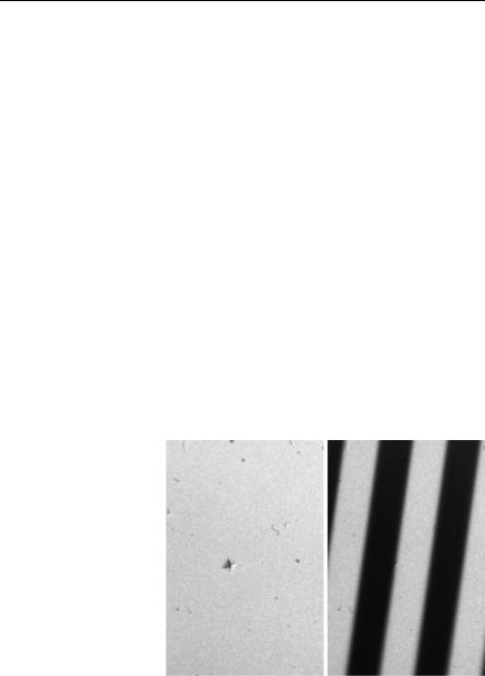
Fig. 3.6 (Left) an image of the object with surface defects. (Right) An image of the object when a Gray code pattern is projected. Figure courtesy of NRC Canada
between the projector fringes and the camera pixels. Figure 3.6 contains an example of a Gray code pattern. Usually, the image in the camera of the narrowest projector fringe is many camera pixels wide and all of these pixels have the same code. It is