Материал: [2.1] 3D Imaging, Analysis and Applications-Springer-Verlag London (2012)
164 |
W.A.P. Smith |
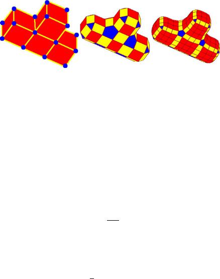
Fig. 4.13 Two iterations of the Doo-Sabin subdivision scheme applied to a T-shaped quadrilateral base mesh. Extraordinary points are shown in blue (reprinted public domain figure)
will create quadrilateral V-faces. Non-quadrilateral faces after one subdivision become extraordinary points in the limit surface. The limit surface is C1 continuous, except at extraordinary points.
4.4.2 Catmull-Clark Scheme
Commencing with a mesh of N vertices, M N = (KN , S), an iteration of the Catmull-Clark subdivision scheme proceeds as follows:
1.For each face f = {i, j, . . . } KN , add a new vertex to the mesh (known as a face point) with a position given by the centroid of the vertices of the face:
vf = |
1 |
vi . |
(4.11) |
f i f |
2. For each edge e = {i, j } KN with adjacent faces f1 and f2, add a new vertex to the mesh (known as an edge point) with a position given by the average of the
edge end points and adjacent face points: |
|
|
|
||
ve = |
1 |
(vi + vj |
+ vf1 |
+ vf2 ). |
(4.12) |
4 |
|||||
The original edge is replaced by two new edges connected to the edge point.
3.Add edges from every edge point ve to their adjacent face points, vf1 and vf2 .
4.For each original point vi , where {i} KN , compute a new position:
vnew |
= |
|
vˆ f + 2vˆ e + (F − 3)vi |
, |
(4.13) |
|
|||||
i |
|
F |
|
||
where vˆ f is the average of the F face points adjacent to the original point and vˆ e is the average of the edge points adjacent to the original point.
4 Representing, Storing and Visualizing 3D Data |
165 |
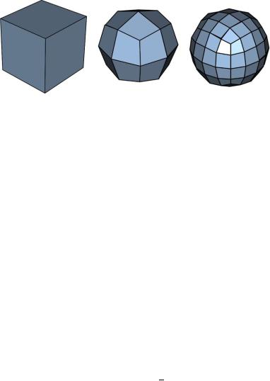
Fig. 4.14 Two iterations of the Catmull-Clark subdivision scheme applied to a cube base mesh. Figure adapted from [74]
The subdivided mesh is composed of quadrilaterals (see Fig. 4.14). In general these will not be planar surfaces. The number of vertices with a degree other than four remains constant over iterations of the subdivision process. These are known as extraordinary points. The limit surface can be shown to be C2 continuous everywhere except at extraordinary vertices, where it is C1 continuous.
4.4.3 Loop Scheme
Unlike the previous two subdivision schemes, Loop’s method operates only on triangular meshes. Commencing with a triangular mesh of N vertices, M N = (KN , S), an iteration of Loop’s scheme proceeds as follows:
1.For every edge e = {i, j } KN a new vertex ve is created as a linear combination of the four vertices comprising the two faces, f1 = {i, j, k1} and f2 = {i, j, k2}, which are adjacent to the edge as shown in Fig. 4.15(a). They are combined using
the following weights:
|
1 |
|
|
1 |
|
|
3 |
3 |
|
|
ve = |
|
vk1 |
+ |
|
vk2 |
+ |
8 vi + |
|
vj . |
(4.14) |
8 |
8 |
8 |
2.The position of each original point is adjusted according to its existing position
and those of its adjacent vertices, as shown in Fig. 4.15(b). For each original point vi , where {i} KN , the new position is given by:
vinew = α |
vj + (1 − di α)vi , |
(4.15) |
|
j Adj(i) |
|
where Adj(i) = {j |{i, j } KN } is the set of vertices adjacent to vi . The constant α is determined by the degree di = Adj(i) and there are many variations
166 |
W.A.P. Smith |
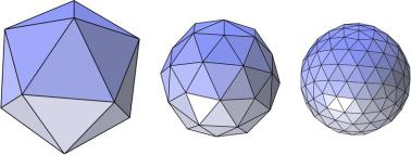
Fig. 4.15 Loop subdivision scheme: (a) creation of an edge vertex; (b) calculating new position for original points; (c) triangulation of new edge points
Fig. 4.16 Two iterations of the Loop subdivision scheme applied to an icosahedron base mesh. Figure adapted from [77]
available. The simplest choice is:
|
|
3 |
|
|
|
|
|
|
|
|
|
if di |
= |
3, |
|
|
|
|
|
|
|
|
|
|
|
||||
α = |
16 |
|
|
|
|
|
|
|
|
|
(4.16) |
|||
1 |
|
[ |
5 |
− ( |
3 |
+ |
1 |
2π 2 |
] |
|
|
|||
|
|
|
|
8 |
8 |
4 cos |
di ) |
if di > |
3. |
|||||
|
|
di |
||||||||||||
3.The subdivided surface is given by connecting the new edge vertices and the updated original vertices as shown in Fig. 4.15(c).
After one subdivision, all vertices have degree six except those which were in the original mesh and had a degree other than six. These are the extraordinary vertices. The limit surface is C2 continuous except at the extraordinary vertices. Figure 4.16 shows loop subdivision applied to an icosahedron base mesh.
4.5 Local Differential Properties
Many useful 3D data processing operations require the computation of local differential properties of a surface. These range from the construction of local features such as spin images [26] to the computation of geodesic paths over a manifold [30].

4 Representing, Storing and Visualizing 3D Data |
167 |
However, most surface representations are discrete and contain only an approximate sampling of the underlying surface. The nature of the representation determines the manner in which these properties are computed.
First order properties of the surface (normal vector and tangent plane) are most commonly used for shading (since surface reflectance is a function of orientation). Interpolation shading uses interpolated surface normals to allow a polygonal approximation of a smooth surface to appear smooth when rendered (see Fig. 4.21(g)). Second order properties (principal curvatures and directions) are often used for local characterization of the surface topology, for example the shape index [32]. Occasionally, even third order properties (directional derivatives of the principal curvatures) can be useful.
For surfaces described in functional form (such as implicit surfaces), differential properties can be computed analytically using differential calculus. On the other hand, discrete representations require the assumption that the underlying surface is smooth and differential properties can only be approximated. Such operators should converge asymptotically to the true result as the sampling density increases.
4.5.1 Surface Normals
For uniformly sampled representations such as voxels and depth maps, differential properties can easily be approximated using finite differences which consider adjacent pixels or voxels, corresponding to the local neighborhood about a point. For example, in the simplest case, the surface gradients in the x and y-directions of a surface represented as a discrete depth map, z(x, y), can be approximated using single forward differences:
∂x z(x, y) ≈
where δx and δy then given by:
z(x + 1, y) − z(x, y) |
, |
∂ |
z(x, y) |
≈ |
z(x, y + 1) − z(x, y) , |
|
|||||
δx |
y |
|
δy |
||
|
|
|
|
|
(4.17) |
are the spacings on the pixel array. The surface normal vector is
n(x, y) |
= |
[∂x z(x, y)∂y z(x, y)1]T |
|
. |
(4.18) |
|
[∂x z(x, y)∂y z(x, y)1]T |
|
|||||
|
|
|
Note that computing gradients using only forward differences results in high sensitivity to noise. For this reason, a window about each pixel can be used in conjunction with an appropriate filter to provide a more stable estimate of the gradients [45].
In the case of an arbitrary triangular mesh, such a simple approach is not possible. If the surface is truly piecewise planar, then it is enough to associate a face normal with each triangular facet. For a face composed of vertices v1, v2 and v3, the face normal is given by:
n |
f = |
(v1 |
− v2) × (v1 |
− v3) |
. |
(4.19) |
|
|
|
||||
|
(v1 − v2) × (v1 − v3) |
|
||||
168 |
W.A.P. Smith |
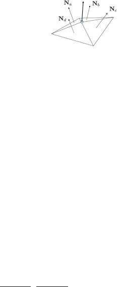
Fig. 4.17 Computation of vertex normal by averaging adjacent face normals
For the normal to be directed to the outside of the object, the vertices must be ordered in an anticlockwise sense when viewed from the outside.
More commonly, the underlying surface is assumed smooth and the surface normal is approximated at each vertex. There are a number of alternative approaches to computing vertex normals [25], which are based on weighted averages of the adjacent facet normals (see Fig. 4.17).
Consider a vertex whose incident edges in anticlockwise order are given by the sequence e1, . . . , en . The first edge is repeated at the end of the sequence so e1 = en. The most well known method which is very efficient to compute uses triangle areas as weights. The area weighted normal to a facet defined by edges ei and ei+1 is given simply by ei × ei+1. Hence, the area weighted vertex normal is:
n−1 |
|
nvArea = ei × ei+1. |
(4.20) |
i=1 |
|
Note that this result requires normalization back to unit length. The efficiency of this approach lies in the fact that the cross product computation factors in the area weight at no extra computational cost. In particular, no trigonometric calculations are required. The downside to this approach is that a triangle with large area but small angle between the edges incident on the vertex contributes disproportionately to the result. This can lead to highly inaccurate normals under certain circumstances and the result depends heavily on the mesh triangulation (see [41] for an example).
An alternative, originally proposed by Thürmer and Wüthrich [70] uses the angle between pairs of edges incident on a vertex as the weight:
|
Angle |
n−1 |
|
ei |
· |
ei 1 |
ei |
× |
ei |
|
1 |
|
|
n |
|
arccos |
|
|
+ |
|
|
+ |
|
. |
(4.21) |
||
|
|
ei ei+1 ei |
× ei+1 |
||||||||||
|
v |
= i 1 |
|
|
|
||||||||
|
|
= |
|
|
|
|
|
|
|
|
|
|
|
Again, the result requires normalization. This approach is relatively simple and accurate but requires trigonometric calculations so is unsuitable for applications involving real-time computation of vertex normals (for example interactive rendering of a deforming surface).
A method proposed by Max [41] offers a compromise. It does not require trigonometric calculations, but is more stable in the special cases where area weighting performs badly. The weight is comprised of the sine of the angle between edge vectors