Материал: [2.1] 3D Imaging, Analysis and Applications-Springer-Verlag London (2012)
204 |
|
|
|
A.M. Bronstein et al. |
|
Table 5.2 Comparison of 3D feature descriptors |
|
|
|
|
|
|
|
|
|
|
|
Descriptor |
Representation |
Invariance |
|
|
|
|
|
|
|
|
|
|
|
Scale |
Rigid |
Bending |
Topology |
|
|
|
|
|
|
Gaussian curvature |
Any |
No |
Yes |
Yes |
Approxc |
Shape index [43] |
Any |
Yes |
Yes |
No |
Approxc |
Integral volume [34] |
Volume, Mesha |
No |
Yes |
No |
Approxc |
Local histograms [66] |
Any |
Nob |
Yes |
Yes |
Nob |
HKS [81] |
Any |
No |
Yes |
Yes |
Approxc |
SIHKS [20] |
Any |
Yes |
Yes |
Yes |
Approxc |
CHKS [47] |
Any+Texture |
Yes |
Yes |
Yes |
Approxc,h |
VHKS [68] |
Volume, Mesha |
No |
Yes |
Yes |
Approxc |
Spin image [39] |
Any |
Noi |
Yes |
Nog |
Yes |
Shape context [5] |
Any |
No |
Yes |
No |
Yes |
MeshHOG [87] |
Mesh (+Texture) |
Yesd |
Yes |
Approxe |
Approxd |
Conformal factor [6] |
Mesh |
No |
Yes |
Yes |
Nof |
aInvolving mesh rasterization
bAssuming geodesic distances. Different invariance properties can be achieved using diffusion or commute-time distances
cPoint-wise connectivity changes have only a local effect and do not propagate to distant descriptors
dIf photometric texture is used; in general, depending on the texture choice
eTriangulation-dependent
fDefined for shapes with fixed topology (e.g. watertight)
gCan be made approximately invariant using small support
hThe use of photometric information can reduce the sensitivity to topological noise compared to HKS
iCan be made scale invariance as in [44]
Finally, some authors [34] make a distinction between high-dimensional (or rich) and low-dimensional descriptors. The former refers to descriptors providing a fairly detailed description of the shape properties around the point such as [5, 39], while the latter computes only a few values per point and typically are curvature-like quantities such as shape index [42] and curvedness [43]. We find this division somewhat misleading, as there is no direct relation between the descriptor “richness” and dimensionality (recent works in computer vision on descriptor hashing and dimensionality reduction [79] demonstrate that rich descriptors such as SIFT can be compactly represented in much lower dimensions without losing much information). The question whether the “richness” of a descriptor is sufficient depends in general on the application and the data.
Table 5.2 summarizes the theoretical properties of known descriptors, some of which are detailed in what follows. The invariance properties of many descriptors were evaluated quantitatively in the SHREC robust feature detection and description
5 Feature-Based Methods in 3D Shape Analysis |
205 |
benchmark [12], testing the descriptor variability under simulated transformations of different types (non-rigid bending, different types of noise, holes, etc.).
We devote particular attention in this section to different varieties of the recently introduced heat kernel signatures, which we consider to be one of the most versatile descriptors currently available, possessing provable invariance properties, as well as a promising and interesting field for future research.
5.4.2 Curvature-Based Descriptors (HK and SC)
The simplest and perhaps earliest shape descriptors based on curvature (also referred to as HK descriptors) were introduced by Besl [8, 9]. The combination of the mean curvature H = 12 (κ1 + κ2) and the Gaussian curvature K = κ1 · κ2 allow the classification of the type of a local surface patch as saddle valley (K, H < 0), saddle ridge (K < 0, H > 0), concave or convex cylinder (K = 0, H < 0 and K = 0, H > 0, respectively), concave or convex ellipsoid (K > 0, H < 0 and K > 0, H > 0, respectively), or plane (K = H = 0). The values of H and K depend on the shape scale.
Koenderink and van Doorn [43] defined a different descriptor (referred to as SC) which decouples the type and strength of local shape curvature as follows: The
shape index S |
2 |
atan( κ1 |
+κ2 ) is a scale-invariant continuous gradation of concave |
||
|
|||||
= π |
κ1 |
− |
|||
κ2 |
|||||
(−1 < S < −0.5), hyperbolic (−0.5 < S < 0.5) and convex (0.5 < S < 1) shapes. |
|||||
|
|
|
|||
The curvedness C = |
(κ12 + κ22)/2 measures how strong the curvature of a particu- |
||||
lar local shape type is at a point. Planar shapes have indeterminate shape index and can be determined from the curvedness C = 0.
Both the HK and SC descriptors make use of the mean curvature, which is not intrinsic and hence not deformation invariant.
5.4.3 Spin Images
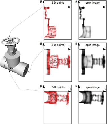
The spin image descriptor [2, 3, 39] represents the neighborhood of a point on a shape by fitting an oriented coordinate system at the point. The local system of cylindrical coordinates at point x is defined using the normal and tangent plane: the radial coordinate α defined as the perpendicular distance to the line through the surface normal n(x), and the elevation coordinate β, defined as the signed perpendicular distance to the tangent plane. The cylindrical angular coordinate is omitted because it cannot be defined robustly and unambiguously on many surface patches, such as those where the curvature is the similar in all directions.
A spin image is a histogram of points in the support region represented in α, β coordinates. The bins can be in linear or logarithmic scale. The support region is defined by limiting the range of the values of α and β (thus looking at points y within some distance from x) and requiring that cos−1 n(x), n(y) < ε (limiting
206 |
A.M. Bronstein et al. |
Fig. 5.4 Example of spin image descriptor computation. Figure reproduced from [38] with permission from Andrew E. Johnson
self occlusion artifacts). The histogram can be represented as a 2D image, hence the name of the descriptor (Fig. 5.4).
The spin image is applicable to any shape representation in which the point coordinates are explicitly given and normals and tangent planes can be computed (e.g., meshes or point clouds). Because of dependence on the embedding coordinates, such a descriptor is not deformation-invariant.
5.4.4 Shape Context
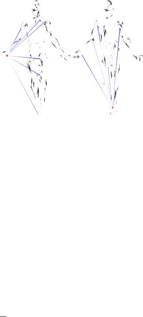
The concept of the shape context descriptor was first introduced in [5] for image analysis, though it is directly applicable to 3D shapes [46]. The shape context describes the structure of the shape as relations between a point to the rest of the points.
5 Feature-Based Methods in 3D Shape Analysis |
207 |
Fig. 5.5 Example of shape context computation. Shown in red is the reference point x, and in blue the rays y − x
Given the coordinates of a point x on the shape, the shape context descriptor is constructed as a histogram of the direction vectors from x to the rest of the points, y − x. Typically, a log-polar histogram is used. The descriptor is applicable to any shape representation in which the point coordinates are explicitly given, such as mesh, point cloud, or volume. Such a descriptor is not deformation-invariant, due to its dependence on the embedding coordinates. An example of shape context computation is shown in Fig. 5.5.
5.4.5 Integral Volume Descriptor
The integral volume descriptor, used in [34], is an extension to 3D shapes of the concept of integral invariants introduced for image description in [54]. Given a solid object Ω with a boundary X = ∂Ω , the descriptor measures volume contained in a ball of fixed radius r ,
Vr (x) = |
dx. |
(5.29) |
|
Br (x)∩Ω |
|
If Br (x) ∩ Ω is simply connected, the volume descriptor can be related to the mean curvature H (x) as Vr (x) = 23π r3 − π4 H r4 + O (r5) [34]. Since the mean curvature is not intrinsic, the descriptor is sensitive to deformations of the shape. Varying the value of r , a multi-scale descriptor can be computed. Numerically, the descriptor is efficiently computed in a voxel representation of the shape, by means of convolution with the ball mask.
208 |
A.M. Bronstein et al. |
5.4.6 Mesh Histogram of Gradients (HOG)
MeshHOG [87] is a shape descriptor emulating SIFT-like image descriptors [51], referred to as histograms of gradients or HOG. The descriptor assumes the shape in mesh representation and in addition to be given some function f defined on the mesh vertices. The function can be either photometric information (texture) or a geometric quantity such as curvature. The descriptor at point x is computed by creating a local histogram of gradients of f in an r -ring neighborhood of x. The gradient f is defined extrinsically as a vector in R3 but projected onto the tangent plane at x which makes it intrinsic. The descriptor support is divided into four polar slices (corresponding to 16 quadrants in SIFT). For each of the slices, a histogram of 8 gradient orientations is computed. The result is a 32-dimensional descriptor vector obtained by concatenating the histogram bins.
The MeshHOG descriptor works with mesh representations and can work with photometric or geometric data or both. It is intrinsic in theory, though the specific implementation in [87] depends on triangulation.
5.4.7 Heat Kernel Signature (HKS)
The heat kernel signature (HKS) was proposed in [81] as an intrinsic descriptor based on the properties of heat diffusion and defined as the diagonal of the heat kernel. Given some fixed time values t1, . . . , tn, for each point x on the shape, the HKS is an n-dimensional descriptor vector
p(x) = kt1 (x, x), . . . , ktn (x, x) . |
(5.30) |
Intuitively, the diagonal values of the heat kernel indicate how much heat remains at a point after certain time (or alternatively, the probability of a random walk to remain at a point if resorting to the probabilistic interpretation of diffusion processes) and is thus related to the “stability” of a point under diffusion process.
The HKS descriptor is intrinsic and thus isometry-invariant, captures local geometric information at multiple scales, is insensitive to topological noise, and is informative (if the Laplace-Beltrami operator of a shape is non-degenerate, then any continuous map that preserves the HKS at every point must be an isometry). Since the HKS can be expressed in the Laplace-Beltrami eigenbasis as
kt (x, x) |
= |
e−t λi φ |
2 |
(x), |
(5.31) |
|
|
i |
|
|
i≥0
it is easily computed across different shape representations for which there is a way to compute the Laplace-Beltrami eigenfunctions and eigenvalues.