Материал: [2.1] 3D Imaging, Analysis and Applications-Springer-Verlag London (2012)
5 Feature-Based Methods in 3D Shape Analysis |
209 |
|||||
|
|
|
|
|
|
|
|
|
|
|
|
|
|
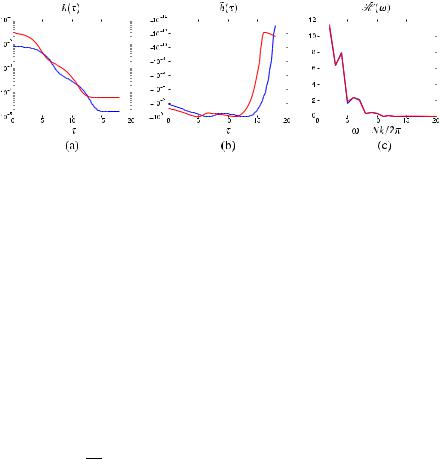
Fig. 5.6 Construction of the Scale-Invariant HKS: (a) we show the HKS computed at the same point, for a shape that is scaled by a factor of 11 (blue dashed plot); please notice the log-scale.
(b) The signal ˜ , where the change in scale has been converted into a shifting in time. (c) The h(τ )
first 10 components of |H˜ (ω)| for the two signals; the descriptors computed at the two different scales are virtually identical
5.4.8 Scale-Invariant Heat Kernel Signature (SI-HKS)
A disadvantage of the HKS is its dependence on the global scale of the shape. If X is globally scaled by β, the corresponding HKS is β−2kβ−2t (x, x). In some cases, it is possible to remove this dependence by global normalization of the shape.
A scale-invariant HKS (SI-HKS) based on local normalization was proposed in [20]. Firstly, the heat kernel scale is sampled logarithmically with some basis α, denoted here as k(τ ) = kατ (x, x). In this scale-space, the heat kernel of the scaled shape becomes k (τ ) = a−2k(τ + 2 logα a) (Fig. 5.6a). Secondly, in order to remove the dependence on the multiplicative constant a−2, the logarithm of the signal followed by a derivative w.r.t. the scale variable is taken,
d
dτ
Denoting
˜
k(τ
log k (τ ) = |
|
d |
|
|
−2 log a + log k(τ + 2 logα a) |
|||||||||||
|
|
|
||||||||||||||
dτ |
||||||||||||||||
|
|
|
= |
|
d |
|
|
log k(τ |
+ 2 logα a) |
|
|
|
||||
|
|
|
|
|
|
|
|
|
||||||||
|
|
|
dτ |
|
|
|
||||||||||
|
|
|
|
|
|
|
d |
k(τ + 2 logα a) |
|
|
|
|||||
|
|
|
= |
|
|
dτ |
|
|
|
|||||||
|
|
|
|
|
|
. |
|
|
|
|||||||
|
|
|
|
|
k(τ + 2 logα a) |
|
|
|
||||||||
|
|
d |
k(τ ) |
|
|
|
− |
i≥0 |
λi ατ log αe−λi ατ |
φ2 |
(x) |
|||||
|
|
dτ |
|
|
|
|||||||||||
) = |
|
|
|
= |
|
|
i |
|
, |
|||||||
|
h(τ ) |
|
|
|
|
i≥0 e−λi ατ φi2(x) |
|
|
||||||||
(5.32)
(5.33)
|
˜ |
|
|
|
|
|
˜ |
(τ ) |
= |
˜ |
+ |
2 log |
α |
|
as a |
|
one thus has a new function k |
which transforms as k |
|
k(τ |
|
a) |
|||||||||||
result of scaling (Fig. 5.6b). Finally, by applying the Fourier transform to |
˜ |
, the |
||||||||||||||
|
|
|
|
|
|
|
|
|
|
|
|
|
|
|
k |
|
shift becomes a complex phase, |
|
˜ |
|
|
= |
˜ |
|
|
|
|
|
|
|
|
||
˜ |
|
= |
|
|
|
|
|
|
|
|
|
|||||
F k |
(ω) |
|
|
K |
|
(ω) |
|
K (ω)e−j ω2 logα a , |
|
|
|
|
(5.34) |
|||
210 |
A.M. Bronstein et al. |
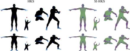
Fig. 5.7 Top: three components of the HKS (left) and the proposed SI-HKS (right), represented as RGB color and shown for different shape transformations (null, isometric deformation+scale, missing part, topological transformation). Bottom: HKS (left) and SI-HKS (right) descriptors at three points of the shape (marked with red, green, and blue). Dashed line shows the null shape descriptor
and taking the absolute value in the Fourier domain (Fig. 5.6c),
˜ |
(ω) |
= |
˜ |
(5.35) |
K |
|
K (ω) , |
produces a scale-invariant descriptor (Fig. 5.7).
5.4.9 Color Heat Kernel Signature (CHKS)
If, in addition, photometric information is available, given in the form of texture α : X → C in some m-dimensional colorspace C (e.g. m = 1 in case of grayscale texture and m = 3 in case of color texture), it is possible to design diffusion processes that take into consideration not only geometric but also photometric information [47, 77]. For this purpose, let us assume the shape X to be a submanifold of some (m + 3)-dimensional manifold E = R3 × C with the Riemannian metric tensor g, embedded by means of a diffeomorphism ξ : X → ξ(X) E . A Riemannian metric on the manifold X induced by the embedding is the pullback metric
(ξ g)(r, s) = g(dξ(r), dξ(s)) for r, s Tx X, where dξ : Tx X → Tξ(x)E is the differential of ξ , and T denotes the tangent space. In coordinate notation, the pullback metric is expressed as (ξ g)μν = gij ∂μξ i ∂ν ξ j , where the indices i, j = 1, . . . , m + 3 denote the embedding coordinates.
The structure of E is to model joint geometric and photometric information. The geometric information is expressed by the embedding coordinates ξg =
(ξ 1, . . . , ξ 3); the photometric information is expressed by the embedding coordinates ξp = (ξ 4, . . . , ξ 3+m) = (α1, . . . , αm). In a simple case when C has a Euclidean structure (for example, the Lab colorspace has a natural Euclidean metric),
the pullback metric boils down to (ξ g)μν
5 Feature-Based Methods in 3D Shape Analysis |
211 |
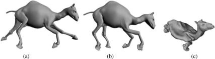
Fig. 5.8 Volumetric (a, b) and boundary (c) isometric deformations of a camel shape. Figure adapted from [80]. According to [68], volume isometries are a better model of physical objects deformation than boundary isometries
The Laplace-Beltrami operator associated with such a metric gives rise to a heat diffusion equation which takes into consideration both the geometry and the color of the object (simplistically put, the heat flows more slowly across different colors). This, in turn, allows the definition of a color-sensitive HKS (CHKS) that merges geometric and photometric information [47].
5.4.10 Volumetric Heat Kernel Signature (VHKS)
So far, we have considered the shape as a 2D boundary surface of a 3D physical object and represented the deformations of the object as deformation of the 2D surface. While physically realistic transformations of reasonably inelastic objects can be modeled as isometries of the 2D boundary surface (“boundary isometries”), the converse is not true: one can easily think of a transformation that preserves the metric structure of the object boundary, but not the volume (Fig. 5.8). Such transformations are not physically realistic, as they change the object volume or mass. However, all intrinsic descriptors we have discussed (including the HKS) would be invariant to such boundary isometries and thus have “too much invariance”.
A different approach is to consider shapes as volumes and require invariance to transformations that preserve the metric structure inside the volume (“volume isometries”). Such descriptors are called volumetric. The idea of the heat kernel descriptor can be applied to volumetric shape representations [68]. In this case, given a solid object Ω , the heat diffusion inside the volume is given by the heat equation
with Neumann boundary conditions on the boundary ∂Ω , |
|
|||
+ |
∂ |
U (x, t ) = 0, |
x int(Ω), |
|
|
(5.36) |
|||
∂t |
||||
U (x, t ), n(x) = 0, |
x ∂Ω |
|
||
where n is the normal to the boundary surface ∂Ω , is the positive-semidefinite Laplacian operator in R3, and U : Ω × [0, ∞) → R is the volumetric heat distribution in Ω . The volumetric heat kernel signature (VHKS) is defined as the diagonal
212 |
A.M. Bronstein et al. |
of the heat kernel of (5.36) at a set of time values t , expressible in the eigenbasis of the Laplacian as
∞ |
|
Kt (x, x) = e−Λl t Φl (x)2, |
(5.37) |
l=0
where Λl , Φl are the eigenvalues and eigenfunctions of the Laplacian operator with the above boundary conditions,
Φl (x) = Λl Φl (x); |
(5.38) |
Φl (x), n(x) = 0, x ∂Ω. |
|
The descriptor can be computed on any volumetric representation of the shape, allowing for efficient computation of the Laplacian eigenvalues and eigenfunctions. For meshes and other surface representations, it is necessary to perform rasterization to convert them into voxel representation [68].
The VHKS is invariant to volumetric isometries of the shape (i.e. deformations that do not change the metric structure inside the shape). Such transformations are necessarily isometries of the boundary ∂Ω , but not vice versa. Thus, VHKS does not have the extra invariance that HKS has.
5.4.11Case Study: Shape Retrieval Using Two Heat Kernel Descriptors (HKS and SI-HKS)
We conclude this section with a case study comparing the performance of two descriptors on a shape retrieval application using a “bags of features”. For additional details on this application, the reader is referred to Chap. 7. A bag of features is a histogram of vector-quantized descriptors, which allows an efficient computation of similarity between shapes, boiling down to the comparison of two histograms. The bag of features inherits the invariance of the underlying local feature descriptor used for its construction. Thus, the choice of the descriptor is crucial for obtaining desired invariance.
In this test case, we used the cotangent weight scheme to discretize the surface Laplace-Beltrami operator; the heat kernel h was approximated using k = 100 largest eigenvalues and eigenvectors. For HKS, we used six scales 1024, 1351, 1783, 2353, 3104 and 4096; for the SI-HKS, we used an exponential scale-space with base α = 2 and τ ranging from 1 to 25 with increments of 1/16. After applying logarithm, derivative, and Fourier transform, the first 6 lowest frequencies were used as the local descriptor. SHREC 2010 dataset was used. The query set consisted of shapes from the dataset undergoing different transformations. Only a single correct match exists in the database, and ideally, it should be the first one.
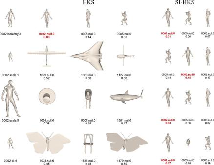
An example of retrieval using bags of features built from HKS and SI-HKS descriptors is shown in Fig. 5.9. It clearly shows the failure of HKS-based bags of
5 Feature-Based Methods in 3D Shape Analysis |
213 |
Fig. 5.9 Retrieval results using bags of features computed with HKS and SI-HKS, tested on the SHREC’10 robust large-scale shape retrieval dataset. Left: query shapes, middle: first three matches obtained with HKS descriptors, right: first three matches obtained with SI-HKS descriptors. Only a single correct match exists in the database (marked in red), and ideally, it should be the first one
features to correctly find similarity between scaled shapes, which makes the use of SI-HKS preferable over HKS in problems involving arbitrary shape scaling.
5.5 Research Challenges
Current challenges in descriptor research include finding a good proportion between theoretical invariance, discriminativity, sensitivity to noise and computational complexity. A single ideal tradeoff is unlikely to be found, since these parameters heavily depend on the application.
Another important challenge of interest both in 2D image and 3D shape analysis is incorporating spatial relations between features. Most feature descriptors capture only local information of the shape, while it is known that, in many cases, the spatial relations between different features are not less important. For example, on a human hand one would find five similar features corresponding to fingers, while their particular spatial configuration is what makes the object recognizable as a hand. Taking this example ad absurdum, one can think of a “soup of features” which have no clear