Материал: [2.1] 3D Imaging, Analysis and Applications-Springer-Verlag London (2012)

2 Passive 3D Imaging |
39 |
tation as the scene (i.e. not inverted top to bottom and left to right) and this position is shown in the figure.
Despite the apparent simplicity of Fig. 2.1(top), a large part of this chapter is required to present the various aspects of stereo 3D imaging in detail, such as calibration, determining left-to-right image correspondences and dense 3D shape reconstruction. A typical commercial stereo camera, supplied by Videre Design.1 is shown in the center of Fig. 2.1, although many computer vision researchers build their own stereo rigs, using off-the-shelf digital cameras and a slotted steel bar mounted on a tripod. Finally, at the bottom of Fig. 2.1, we show the left and right views of a typical stereo pair taken from the Middlebury webpage [34].
In contrast to stereo vision, structure from motion (SfM) refers to a single moving camera scenario, where image sequences are captured over a period of time. While stereo refers to fixed relative viewpoints with synchronized image capture, SfM refers to variable viewpoints with sequential image capture. For image sequences captured at a high frame rate, optical flow can be computed, which estimates the motion field from the image sequences, based on the spatial and temporal variations of the image brightness. Using the local brightness constancy alone, the problem is under-constrained as the number of variables is twice the number of measurements. Therefore, it is augmented with additional global smoothness constraints, so that the motion field can be estimated by minimizing an energy function [23, 29]. 3D motion of the camera and the scene structure can then be recovered from the motion field.
2.2.2 Single View Approaches
In contrast to these two multiple-view approaches, 3D shape can be inferred from a single viewpoint using information sources (cues) such as shading, texture and focus. Not surprisingly, these techniques are called shape from shading, shape from texture and shape from focus respectively.
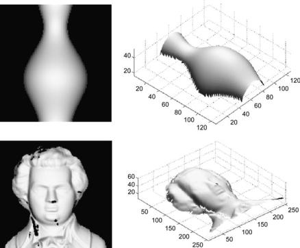
Shading on a surface can provide information about local surface orientations and overall surface shape, as illustrated in Fig. 2.2, where the technique in [24] has been used. Shape from shading [22] uses the shades in a grayscale image to infer the shape of the surfaces, based on the reflectance map which links image intensity with surface orientation. After the surface normals have been recovered at each pixel, they can be integrated into a depth map using regularized surface fitting. The computations involved are considerably more complicated than for multiple-view approaches. Moreover, various assumptions, such as uniform albedo, reflectance and known light source directions, need to be made and there are open issues with convergence to a solution. The survey in [65] reviews various techniques and provides some comparative results. The approach can be enhanced when lights shining from different directions can be turned on and off separately. This technique is
1http://www.videredesign.com.
40 |
S. Se and N. Pears |
Fig. 2.2 Examples of synthetic shape from shading images (left column) and corresponding shape from shading reconstruction (right column)
known as photometric stereo [61] and it takes two or more images of the scene from the same viewpoint but under different illuminations in order to estimate the surface normals.
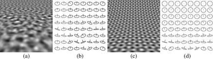
The foreshortening of regular patterns depends on how the surface slants away from the camera viewing direction and provides another cue on the local surface orientation. Shape from texture [17] estimates the shape of the observed surface from the distortion of the texture created by the imaging process, as illustrated in Fig. 2.3. Therefore, this approach works only for images with texture surfaces and assumes the presence of a regular pattern. Shape from shading is combined with shape from texture in [60] where the two techniques can complement each other. While the texture components provide information in textured region, shading helps in the uniform region to provide detailed information on the surface shape.
Shape from focus [37, 41] estimates depth using two input images captured from the same viewpoint but at different camera depths of field. The degree of blur is a strong cue for object depth as it increases as the object moves away from the camera’s focusing distance. The relative depth of the scene can be constructed from
2 Passive 3D Imaging |
41 |
Fig. 2.3 Examples of synthetic shape from texture images (a, c) and corresponding surface normal estimates (b, d). Figure courtesy of [17]
the image blur where the amount of defocus can be estimated by averaging the squared gradient in a region.
Single view metrology [13] allows shape recovery from a single perspective view of a scene given some geometric information determined from the image. By exploiting scene constraints such as orthogonality and parallelism, a vanishing line and a vanishing point in a single image can be determined. Relative measurements of shape can then be computed, which can be upgraded to absolute metric measurements if the dimensions of a reference object in the scene are known.
While 3D recovery from a single view is possible, such methods are often not practical in terms of either robustness or speed or both. Therefore, the most commonly used approaches are based on multiple views, which is the focus of this chapter. The first step to understanding such approaches is to understand how to model the image formation process in the cameras of a stereo rig. Then we need to know how to estimate the parameters of this model. Thus camera modeling and camera calibration are discussed in the following two main sections.
2.3 Camera Modeling
A camera is a device in which the 3D scene is projected down onto a 2D image. The most commonly used projection in computer vision is 3D perspective projection. Figure 2.4 illustrates perspective projection based on the pinhole camera model, where C is the position of the pinhole, termed the camera center or the center of projection. Recall that, although the real image plane is behind the camera center, it is common practice to employ a virtual image plane in front of the camera, so that the image is conveniently at the same orientation as the scene.
Clearly, from this figure, the path of imaged light is modeled by a ray that passes from a 3D world point X through the camera center. The intersection of this ray with the image plane defines where the image, xc , of the 3D scene point, X, lies. We can reverse this process and say that, for some point on the image plane, its corresponding scene point must lie somewhere along the ray connecting the center of projection, C, and that imaged point, xc . We refer to this as back-projecting an image point to an infinite ray that extends out into the scene. Since we do not know

42 |
S. Se and N. Pears |
Fig. 2.4 Projection based on a pinhole camera model where a 3D object is projected onto the image plane. Note that, although the real image plane is behind the camera center, it is common practice to employ a virtual image plane in front of the camera, so that the image is conveniently at the same orientation as the scene
how far along the ray the 3D scene point lies, explicit depth information is lost in the imaging process. This is the main source of geometric ambiguity in a single image and is the reason why we refer to the recovery of the depth information from stereo and other cues as 3D reconstruction.
Before we embark on our development of a mathematical camera model, we need to digress briefly and introduce the concept of homogeneous coordinates (also called projective coordinates), which is the natural coordinate system of analytic projective geometry and hence has wide utility in geometric computer vision.
2.3.1 Homogeneous Coordinates
We are all familiar with expressing the position of some point in a plane using a pair of coordinates as [x, y]T . In general for such systems, n coordinates are used to describe points in an n-dimensional space, Rn. In analytic projective geometry, which deals with algebraic theories of points and lines, such points and lines are typically described by homogeneous coordinates, where n + 1 coordinates are used to describe points in an n-dimensional space. For example, a general point in a plane is described as x = [x1, x2, x3]T , and the general equation of a line is given by lT x = 0 where l = [l1, l2, l3]T are the homogeneous coordinates of the line.2 Since the right hand side of this equation for a line is zero, it is an homogeneous equation, and any non-zero multiple of the point λ[x1, x2, x3]T is the same point, similarly any non-zero multiple of the line’s coordinates is the same line. The symmetry in this
2You may wish to compare lT x = 0 to two well-known parameterizations of a line in the (x, y) plane, namely: ax + by + c = 0 and y = mx + c and, in each case, write down homogeneous coordinates for the point x and the line l.
2 Passive 3D Imaging |
43 |
equation is indicative of the fact that points and lines can be exchanged in many theories of projective geometry; such theories are termed dual theories. For example, the cross product of two lines, expressed in homogeneous coordinates, yields their intersecting point, and the cross-product of a pair of points gives the line between them.
Note that we can easily convert from homogeneous to inhomogeneous coordinates, simply by dividing through by the third element, thus [x1, x2, x3]T maps to
[ x1 , x2 ]T . A key point about homogeneous coordinates is that they allow the relevant
x3 x3
transformations in the imaging process to be represented as linear mappings, which of course are expressed as matrix-vector equations. However, although the mapping between homogeneous world coordinates of a point and homogeneous image coordinates is linear, the mapping from homogeneous to inhomogeneous coordinates is non-linear, due to the required division.
The use of homogeneous coordinates fits well with the relationship between image points and their associated back-projected rays into the scene space. Imagine a mathematical (virtual) image plane at a distance of one metric unit in front of the center of projection, as shown in Fig. 2.4. With the camera center, C, the homogeneous coordinates [x, y, 1]T define a 3D scene ray as [λx, λy, λ]T , where λ is the unknown distance (λ > 0) along the ray. Thus there is an intuitive link between the depth ambiguity associated with the 3D scene point and the equivalence of homogeneous coordinates up to an arbitrary non-zero scale factor.
Extending the idea of thinking of homogeneous image points as 3D rays, consider the cross product of two homogeneous points. This gives a direction that is the normal of the plane that contains the two rays. The line between the two image points is the intersection of this plane with the image plane. The dual of this is that the cross product of two lines in the image plane gives the intersection of their associated planes. This is a direction orthogonal to the normals of both of these planes and is the direction of the ray that defines the point of intersection of the two lines in the image plane. Note that any point with its third homogeneous element zero defines a ray parallel to the image plane and hence meets it at infinity. Such a point is termed a point at infinity and there is an infinite set of these points [x1, x2, 0]T that lie on the line at infinity [0, 0, 1]T ; Finally, note that the 3-tuple [0, 0, 0]T has no meaning and is undefined. For further reading on homogeneous coordinates and projective geometry, please see [21] and [12].
2.3.2 Perspective Projection Camera Model
We now return to the perspective projection (central projection) camera model and we note that it maps 3D world points in standard metric units into the pixel coordinates of an image sensor. It is convenient to think of this mapping as a cascade of three successive stages:
1.A 6 degree-of-freedom (DOF) rigid transformation consisting of a rotation, R (3 DOF), and translation, t (3 DOF), that maps points expressed in world coordinates to the same points expressed in camera centered coordinates.