Материал: [2.1] 3D Imaging, Analysis and Applications-Springer-Verlag London (2012)

We denote Pp as the 3 × 4 perspective projection matrix, defined by the value of f , in the above equation. If we consider an abstract image plane at f = 1, then points on this plane are termed normalized image coordinates4 and from Eq. (2.2), these are given by

2.3.2.3 Camera Modeling: Image Sampling

Typically, the image on the image plane is sampled by an image sensor, such as a CCD or CMOS device, at the locations defined by an array of pixels. The final part of camera modeling defines how that array is positioned on the [xc , yc ]T image plane, so that pixel coordinates can be generated. In general, pixels in an image sensor are not square and the number of pixels per unit distance varies between the xc and yc directions; we will call these scalings mx and my . Note that pixel positions have their origin at the corner of the sensor and so the position of the principal point (where the principal axis intersects the image plane) is modeled with pixel coordinates [x0, y0]T . Finally, many camera models also cater for any skew,5 s, so that the mapping into pixels is given by:

We denote Pc as the 3 × 3 projective matrix defined by the five parameters mx , my , s, x0 and y0 in the above equation.

2.3.2.4 Camera Modeling: Concatenating the Projective Mappings

We can concatenate the three stages described in the three previous subsections to give

λx = Pc Pp Pr X

or simply

where λ is non-zero and positive. We note the following points concerning the above equation

4We need to use a variety of image coordinate normalizations in this chapter. For simplicity, we will use the same subscript n, but it will be clear about how the normalization is achieved.

5Skew models a lack of orthogonality between the two image sensor sampling directions. For most imaging situations it is zero.

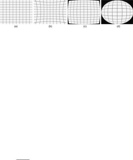
Fig. 2.5 Examples of radial distortion effects in lenses: (a) No distortion (b) Pincushion distortion (c) Barrel distortion (d) Fisheye distortion

2.3.3 Radial Distortion

Typical cameras have a lens distortion, which disrupts the assumed linear projective model. Thus a camera may not be accurately represented by the pinhole camera model that we have described, particularly if a low-cost lens or a wide field-of- view (short focal length) lens such as a fisheye lens is employed. Some examples of lens distortion effects are shown in Fig. 2.5. Note that the effect is non-linear and, if significant, it must be corrected so that the camera can again be modeled as a linear device. The estimation of the required distortion parameters to do this is often encompassed within a camera calibration procedure, which is described in Sect. 2.4. With reference to our previous three-stage development of a projective camera in Sect. 2.3.2, lens distortion occurs at the second stage, which is the 3D to 2D projection, and this distortion is sampled by the image sensor.

Detailed distortion models contain a large number of parameters that model both radial and tangential distortion [7]. However, radial distortion is the dominant factor and usually it is considered sufficiently accurate to model this distortion only, using a low-order polynomial such as:

where [xn, yn]T is the undistorted image position (i.e. that obeys our linear projection model) in normalized coordinates, [xnd , ynd ]T is the distorted image position in normalized coordinates, k1 and k2 are the unknown radial distortion parameters,

and r = xn2 + yn2. Assuming zero skew, we also have

that r is still defined in normalized image coordinates and so a non-unity aspect ratio (mx = my ) in the image sensor does not invalidate this equation. Also note that both Eq. (2.6) and Fig. 2.5 indicate that distortion increases away from the center of the image. In the barrel distortion, shown in Fig. 2.5(c), distortion correction requires that image points are moved slightly towards the center of the image, more so if they are near the edges of the image. Correction could be applied to the whole image, as

in dense stereo, or just a set of relevant features, such as extracted corner points. Clearly, the latter process is computationally cheaper.

Now that we have discussed the modeling of a camera’s image formation process in detail, we now need to understand how to estimate the parameters within this model. This is the focus of the next section, which details camera calibration.

2.4 Camera Calibration

Camera calibration [8] is the process of finding the parameters of the camera that produced a given image of a scene. This includes both extrinsic parameters R, t and intrinsic parameters, comprising those within the matrix K and radial distortion parameters, k1, k2. Once the intrinsic and extrinsic camera parameters are known, we know the camera projection matrix P and, taking into account of any radial distortion present, we can back-project any image pixel to a 3D ray in space. Clearly, as the intrinsic camera calibration parameters are tied to the focal length, changing the zoom on the lens would make the calibration invalid. It is also worth noting that calibration is not always required. For example, we may be more interested in approximate shape, where we need to know what objects in a scene are co-planar, rather than their absolute 3D position measurements. However, for stereo systems at least, camera calibration is commonplace.

Generally, it is not possible for an end-user to get the required calibration information to the required accuracy from camera manufacturer’s specifications and external measurement of the position of cameras in some frame. Hence some sort of camera calibration procedure is required, of which there are several different categories. The longest established of these is photogrammetric calibration, where calibration is performed using a scene object of precisely known physical dimensions. Typically, several images of a special 3D target, such as three orthogonal planes with calibration grids (chessboard patterns of black and white squares), are captured and precise known translations may be used [58]. Although this gives accurate calibration results, it lacks flexibility due to the need for precise scene knowledge.

At the other end of the spectrum is self-calibration (auto-calibration) [21, 35], where no calibration target is used. The correspondences across three images of the same rigid scene provide enough constraints to recover a set of camera parameters which allow 3D reconstruction up to a similarity transform. Although this approach is flexible, there are many parameters to estimate and reliable calibrations cannot always be obtained.

Between these two extremes are ‘desktop’ camera calibration approaches that use images of planar calibration grids, captured at several unknown positions and orientations (i.e. a single planar chessboard pattern is manually held at several random poses and calibration images are captured and stored). This gives a good compromise between the accuracy of photogrammetric calibration and the ease of use of self-calibration. A seminal example is given by Zhang [64].

Although there are a number of publicly available camera calibration packages on the web, such as the Caltech camera calibration toolbox for MATLAB [9] and in