Материал: [2.1] 3D Imaging, Analysis and Applications-Springer-Verlag London (2012)

6 3D Shape Registration |
255 |
6.7.3 Minimization Procedure
The DLM-ICP cost function (6.24) is a sum of squared residuals, nonlinearly depending on the unknowns in M. Therefore, as in Sect. 6.6, the Levenberg-Marquardt algorithm can be used. In order to provide partial derivatives of the residuals through a Jacobian matrix, all five terms in the cost function are separately differentiated and stacked as:
J T = JdT JbT JsT JtT JxT , |
(6.33) |
where JdNm×3Nm , JbNB ×3Nm , Js3Nm ×3Nm , JtNm×3Nm , Jxξ ×3Nm , are related to the global attraction, boundary attraction, spatial smoothness, temporal smoothness and non-
extensibility terms respectively, and ξ = size(N (M)). In particular, the Jacobians of global and boundary attraction terms are estimated by finite differences through distance transform, as described in Sect. 6.6.
Note that, in this case, since the Hessian matrix11 H = JTJ + λI must be inverted at each LM iteration, the problem is not tractable if the number of model points is too high (if the deformation field is too dense). One advantage of the proposed approach is that the Jacobian matrix J is very sparse. Thus, it uses the sparsity to speed up each iteration using the technique in [68]. In particular, a sparse Cholesky factorization package can be used, as in the Matlab ‘mldivide’ function.
6.7.4 Summary of the Algorithm
The DLM-ICP algorithm can be summarized as follows:
1.Choose the model-size R × C (for instance, 10 × 10)
2.Initialize the template-model M0
3.For each data-frame Di
a.Extract data boundary BD
b.Set Mi = Mi−1 to initialize the LM algorithm
c.Apply LM-ICP to estimate Mi by minimizing the error function
d.Goto 3.
Step 3.c is described in Sect. 6.6.4. Here, the unknown is a = Mi , the error function E(Mi ) is defined by Eq. (6.24), and the Jacobian J is defined by Eq. (6.33).
6.7.5 Experiments
In the following experiment, the sensor is a real-time passive-stereo system.12 The sensor acquires images at 25 FPS (frames-per-second) and provides both intensity
11The damped Gauss-Newton approximation to the true Hessian matrix.
12Data courtesy of eVS (http://www.evsys.net).
256 |
U. Castellani and A. Bartoli |
Fig. 6.17 Data acquisition: intensity image of the blanket (left), image-boundary (center), and the 3D point cloud (right)
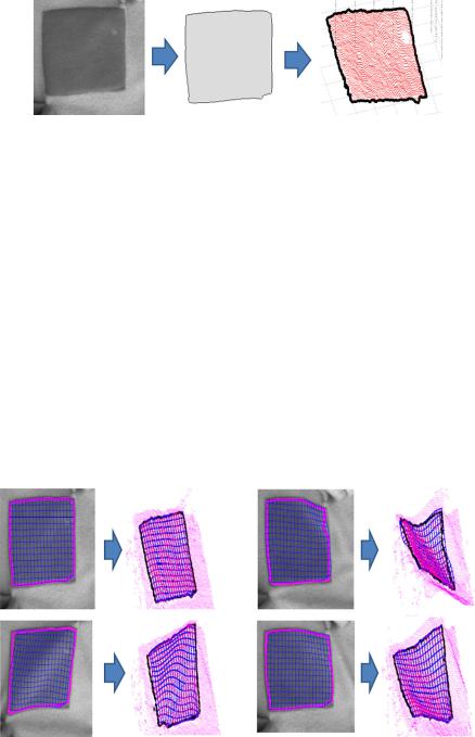
(i.e. 2D) and 3D information. The deformation of a portion of a blanket is modeled. Figure 6.17 shows a picture of the blanket. Intensity information is used to segment the boundary; more precisely, only the portion delimited by the dark square is considered. Figure 6.17 also shows the image-boundary extracted by combining a binary image segmentation method with 2D morphological operators and depicts the 3D data (i.e. the selected point cloud and 3D boundary).
The sequence is made of 100 point clouds. A model of size R = 15 and C = 20 is used. Model initialization M0 is carried out by lying the model-grid on a plane which is fitted to the extracted point cloud. Model initialization is employed in the first frame only. Then, each iteration uses the output of the previous one as an initial condition. Note that a higher value of λb is necessary (i.e. λb = 1.5) for a correct convergence of the algorithm to the optimal solution. The other terms are set almost equally to 1. The distance transform parameters are important: the size of the voxels trades off speed and accuracy. In this experiment, the volume is divided into 36 × 36 × 18 voxels. Figure 6.18 shows a selection of the output sequence. For each frame, we visualize: (i) the intensity image with the extracted 2D boundary and the
Fig. 6.18 Blanket sequence: 4 selected frames. For each frame the 2D intensity and the 3D data is visualized. The grid models are shown in 3D space, as well as their projection in the 2D image
6 3D Shape Registration |
257 |
2D projection of the estimated model and (ii) the point cloud, after the region-of- interest selection, evidencing both the 3D boundary and the grid.
The blanket is handled from the bottom-left and upper-right corners, respectively. On the early frames, the blanket is gradually bent toward the square center, then it is strongly stretched, moving the corners far from each other. Finally, in the late frames, random deformations are generated, especially around the corners. Results are satisfying since the fitting is correct for the whole sequence, in spite of the presence of strong occlusions and deformations. The mesh grids are well superimposed on data points maintaining a smooth shape. Nevertheless, the projection of the grids to the 2D images confirms the accuracy of the registration. More details on performance evaluation are available in [19].
6.8 Research Challenges
In general, new challenges of registration methods arise from advances in acquisition procedures. Structure and motion reconstruction techniques are now available to provide accurate, sparse or dense reconstructed scenes from 2D images. Largescale scanners are also able to acquire wide scenes. The registration of data coming from these procedures is challenging due to strong clutter and occlusions. Moreover, as observed before, the object to be registered may be very small with respect to the whole scene. An important issue is the local scale estimation of scene subparts. On the other hand, texture or color information can be also acquired by the sensor. Therefore, registration can be improved by integrating effectively these additional cues. Another promising direction is the use of machine learning techniques. In particular, new techniques can be exploited, inspired from similar issues already addressed for the 2D domain like face, car or pedestrian detection techniques. Improvements can be achieved by integrating 3D scans and 2D images.
Other problems need to be addressed when real-time scanners are used. In this scenario, objects can move (change their pose) or deform. Therefore, deformable registration techniques should be employed. In particular, all the advances on isometry-invariant point correspondence computation can improve the deformable registration. Other issues are coming from the explosion of data collection. For instance, from real-time scanners a large amount of data can be acquired. In order to avoid exhaustive search some more effective matching strategies can be exploited. Feature based techniques are useful to this aim. In particular, feature point detection and description can reduce drastically the number of analyzed points. Also hierarchical techniques are needed to reduce the search space. Finally, to design a proper surface deformation transform, deformable registration methods can be inspired from 3D animation techniques.
6.9 Concluding Remarks
Registration of 3D data is a well studied problem but new issues still need to be solved. The ICP algorithm is the current standard method, since it works well in
258 |
U. Castellani and A. Bartoli |
general and it is easy to implement. Although the basic version is quite limited, several extensions and strong variants have been introduced that allow it to cope with many scenarios. For instance, the techniques described in Sect. 6.2.3 are sufficient to obtain a full model reconstruction of a single object observed from a few dozen viewpoints. However, in more challenging situations, such as in the presence of cluttered or deformable objects, the problem becomes more difficult. The point matching strategy needs to be improved and the transformation function needs to be properly designed. Therefore, more advanced techniques need to be employed like those described in Sect. 6.3. In order to give some examples of registration algorithms, three case studies were reported. Case study 1 shows how, in practice, a robust outlier rejection strategy can improve the accuracy of registration and estimate the overlapping area. Case study 2 exploits general Levenberg-Marquardt optimization to improve the basic ICP algorithm. In particular, the advantage of using the distance transform is clearly demonstrated. Finally, case study 3 addresses a more challenging problem, namely deformable registration from real-time acquisition. Also in this case, the Levenberg-Marquardt approach enables the modeling of the expected behavior of surface deformations. In particular, effective data and penalty terms can be encoded easily in the general error function.
New challenging scenarios can be addressed as described in Sect. 6.8 by exploiting recent machine learning and computer vision techniques already successfully employed for the 2D domain, as well as new advances inspired from recent computer animation techniques.
6.10 Further Reading
In order to get a more comprehensive overview of 3D registration methods, the reader can refer to recent surveys [48, 57, 78, 79]. In [78], Ruzinkiewicz et al. have analyzed some variants of the ICP technique, focusing on methods and suggestions to improve the computation speed. An extensive review of registration methods based on the definition of surface shape descriptors can be found in [57]. In [79], Salvi et al. proposed an extensive experimental comparison amongst different 3D pairwise registration methods. They evaluated the accuracy of the results for both coarse and fine registration. More recently, Kaick et al. [48] proposed a survey on shape correspondence estimation by extensively reporting and discussing interesting methods for deforming scenarios.
The reader interested in getting in-depth details on the theoretical evaluation of registration convergence should refer to Pottmann et al.’s work [35, 69]. Convergence is discussed also by Ezra et al. [31] who provided lower and upper bounds on the number of ICP iterations. One of these methods [86] defines a new registration metric called the ‘surface interpenetration measure’. This is in contrast to the mean square error (MSE) employed by classical ICP and the authors claim that this is more effective when attempting to achieve precise alignments. Finally, we have stated already that most of the registration techniques are based on the ICP

6 3D Shape Registration |
259 |
algorithm. However, alternative methods in the literature can be considered, such as those based on Genetic Algorithms [52, 53, 86].
6.11 Questions
1.Give four examples of problem where 3D shape registration is an essential component. In each case, explain why registration is required for their automated solution.
2.Briefly outline the steps of the classical iterative closest point (ICP) algorithm.
3.What is usually the most computationally intensive step in a typical ICP application and what steps can be taken to reduce this?
4.What is the common failure mode of ICP and what steps can be taken to avoid this?
5.What steps can be taken to improve the final accuracy of an ICP registration?
6.Explain why registration in clutter is challenging and describe one solution that has been proposed.
7.Explain why registration of deformable objects is challenging and describe one solution that has been proposed.
8.What advantages does LM-ICP have over classical ICP?
6.12 Exercises
1.Given two partial views very close to each other and an implementation of ICP13 try to register the views by gradually moving the data-view away from the modelview until ICP diverges. Apply the perturbation to both the translational and rotational components. Repeat the exercise, decreasing the overlap area by removing points in the model-view.
2.Implement a pairwise pre-alignment technique based on PCA. Try to check the effectiveness of the pre-alignment by varying the shape of the two views.
3.Implement an outlier rejection technique to robustify ICP registration. Compare the robustness among (i) fixed threshold, (ii) threshold estimated as 2.5σ of the residuals’ distribution from their mean and (iii) threshold estimated with the X84 technique.
4.Compute the Jacobian matrix of LM-ICP by encoding rotation with a unit quaternion.14
5.Modify LM-ICP in order to work with multiple views, given a sequence of 10 views which surround an object such that N10 is highly overlapping N1. The global reference system is fixed on the first view. Estimate the global registration
13Matlab implementation at: http://www.csse.uwa.edu.au/ajmal/code.html.
14Matlab implementation at: http://research.microsoft.com/en-us/um/people/awf/lmicp.