Материал: [2.1] 3D Imaging, Analysis and Applications-Springer-Verlag London (2012)

250 |
U. Castellani and A. Bartoli |
a.compute update ak+1 = ak − (JT J + λI)−1JT ek 7
b.compute E = E(ak+1) − E(ak )
c.If E > 0 then λ = 10λ, goto a. else λ = 101 λ, goto 4.
7.If ek > ν goto 3. else terminate.
Note that ν is a constant which defines the convergence of the algorithm. As already highlighted, the algorithm above is the standard LM algorithm. The crucial components are (i) the choice of unknowns a, (ii) the computation of error vector e and (iii) the computation of the Jacobian matrix J. In particular, the distance transform Dε (x), enables an improvement in the computational efficiency of the error computation and makes the computation of the Jacobian feasible. The starting value a0 can be estimated by employing some of the techniques described in Sect. 6.2.3.1.
6.6.5 Results and Discussion
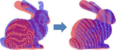
Figure 6.16 shows an example of LM-ICP alignment between two views. In this experiment the emphasis is on the speed of the algorithm, since the accuracy is guaranteed by the fact that the two views are well overlapped. The LM-ICP takes less than 1 s for an LM iteration. A total of 20 iterations has been run to reach convergence. Both the data-view and the model-view have about 40,000 points. Using the basic ICP algorithm the same number of iterations are required but each iteration takes more than 30 s. This confirms that a drastic improvement of speed is observed with LM-ICP, in comparison with basic ICP. Note that a crucial parameter is the grid size. It trades off computational efficiency with memory space. Moreover it requires that the data scan is always inside the volume by requiring large memory space for storage when only a small overlap is observed between the views. Further experiments can be found in [32]. More details on experimental set-up can be found on the LM-ICP website.8 In practice LM-ICP also enlarges the basin of convergence and estimates a more accurate solution (the minimum is reached with 50 % fewer iterations on average, see [32] for more details).
Finally, it is worth noting that LM-ICP can be easily extended to apply many other variants of the ICP. Multi-view registration could also be solved in the LMICP framework.
6.7 Case Study 3: Deformable ICP with Levenberg-Marquardt
In this section, we describe an advanced registration technique: Deformable- Levenberg-Marquardt Iterative Closest Point (DLM-ICP) [19]. DLM-ICP extends
7While we have chosen the identity as the damping matrix, some authors rather choose the diagonal part of the Gauss-Newton Hessian approximation.
8http://research.microsoft.com/en-us/um/people/awf/lmicp.
6 3D Shape Registration |
251 |
Fig. 6.16 LM-ICP. The starting pose (left) and merged views after registration (right)
the LM-ICP approach, introduced in Sect. 6.6, to deformable objects. We focus on continuous smooth surfaces such as the page of a book being turned in front of a range sensor. To this aim, a template model is warped towards the input scans in order to capture surface deformations. In this case, several instances of almost the entire time-varying object are observed rather than different points of view of an object, and the aim of registration is to align the views over time using a registration- by-fitting approach.
The template model introduces a prior on the acquired shape by providing a joint registration and reconstruction of the object with hole-filling and noise removal. The proposed method exploits only geometric information without the extraction of feature points. According to [32], described in Sect. 6.6, registration is modeled as an optimization problem defined by an error function whose global minimum is the sought after solution, estimated by the Levenberg-Marquardt algorithm. The error function introduces the constraint that data points must be close to model points (i.e. the template). As for [32], it explicitly embeds a min operator, thus avoiding the traditional two steps in ICP-like algorithms, through the use of a distance transform. Furthermore, thanks to the flexibility of LM, many other terms are introduced to model different expected behaviors of the deformation, namely surface, and temporal smoothness as well as inextensibility of the surface. Finally, a boundary constraint is introduced to prevent the computed surface from sliding arbitrarily.
We highlight that, with this method, the unknowns are the template model, represented by a planar-mesh that is deformed to fit each point cloud. More specifically, we directly estimate the position of the model-points without imposing any prior about the kind of transformation function that has been applied. In particular, each unknown (i.e. each vertex of the template) influences a very small portion of the error function. Indeed, another interesting property of DLM-ICP is that the Jacobian matrix, involved in the normal equations to be solved at each iteration, is highly sparse for all the terms. This makes the estimation of dense deformation fields tractable and fast.
252 |
U. Castellani and A. Bartoli |
6.7.1 Surface Representation
The sequence of 3D point clouds Di , with Nd
|
|
di,x |
1 |
di,y |
1 |
|
Di |
= |
|
. |
|
. |
|
|
. |
|
. |
|
||
. |
|
. |
|
|||
|
|
x |
|
y |
|
|
|
|
|
di,li |
di,li |
||
= li points each, is represented by:
dz 1
i,
.
. .
.
di,lz i
The unknown model, a = M, has a grid structure and is thus represented by three R × C matrices, giving the grid’s deformation. Each matrix is reshaped in a single vector of size Nm = RC, giving Mi as:
mi,x 1 |
mi,y 1 |
mi,z 1 |
|
. |
. |
. |
|
. |
. |
. |
. |
Mi = . |
. |
. |
|
mx |
my |
mz |
|
i,Nm |
i,Nm |
i,Nm |
|
In practice, the number of data points is much larger than the number of model points (i.e. li Nm). Upon convergence, the algorithm determines, for each model point, if there is a corresponding point in the current point cloud. Points may be missing because of occlusions or corrupted sensor output. This approach has the advantage that it naturally gives the reconstructed surface by interpolating the mesh points. Point cloud registration is obtained by composing the deformation fields. Note that, in contrast to Sect. 6.6, the registration is from model-points to datapoints.
6.7.2 Cost Function
The cost function combines two data and three penalty terms:
E(M) = Eg (M) + λb Eb(M) + λs Es (M) + λt Et (M) + λx Ex (M), |
(6.24) |
where λb , λs λx and λt are weights. Note that we drop the frame index i for purposes
of clarity, and denote as and as ˜ .
Mi M Mi−1 M
The data terms are used to attract the estimated surface to the actual point cloud. The first term Eg is for global attraction, while the second one Eb deals with the boundary. In particular, the boundary term aims at preserving the method against possible sliding of the model along the observed surface. Moreover, these terms must account for possible erroneous points by using robust statistics. The penalty terms are Es , Et and Ex . The first two account for spatial smoothness and temporal smoothness Es respectively. The third one penalizes the surface stress and is related to the non-extensibility of the surface, and therefore to material properties of the surface.
This cost function is minimized in an ICP-like manner, as described in the previous section. All five terms are explained below in detail.

6 3D Shape Registration |
253 |
Data Term: Global Surface Attraction This term globally attracts the model to the data points in a closest point manner [78]. Denoting BM as the set of boundary points in the model, M, where
M |
= |
mx |
my |
mz T , |
i |
= |
1 . . . Nm |
(6.25) |
||
|
|
i |
i |
i |
|
|
|
|||
and BD as the set of boundary points in the data, D, where |
|
|||||||||
D |
= |
dx dy |
dz T , |
i |
= |
1 . . . li |
(6.26) |
|||
|
|
i |
i |
i |
|
|
|
|||
we get the following data term, integrating the model to data points matching step:
min d − m 2, |
(6.27) |
m M\BM d D\BD
where d and m are 3-vectors representing a data and a model point respectively. As we mentioned before, the unknowns are not the rigid transformation parameters (i.e. the classical rotation-translation) but correspond to the whole deformable motion field in M.
An outlier rejection strategy is introduced by defining a robust function ε. Here, the X84 rule is employed [17]. Therefore, Eq. (6.27) is modified so as to get the following robustified data term:
M |
|
|
min |
d − m |
2 . |
(6.28) |
|
Eg ( ) = |
m M\BM |
ε |
d D |
BD |
|
|
|
|
|
\ |
|
|
|
|
|
Data Term: Boundary Attraction This term attracts boundary model points to boundary data points. It is defined in a similar manner to the global attraction term (Eq. (6.28)) except that the sum and min operators are over the boundary points:
E |
M |
|
min |
|
d |
− |
m |
2 . |
(6.29) |
||
|
b ( ) = |
m BM |
ε |
d |
BD |
|
|
|
|
||
|
|
|
|
|
|
|
|
|
|
|
|
Note that the boundaries can be computed by combining edge detection techniques with morphological operators.9 More precisely, from the range image, we detect the portion of the image which is covered by the object we want to track (i.e. a piece of paper), and we impose the condition that boundaries of the model and the observed surface must coincide.
Penalty Term: Spatial Smoothness This term discourages surface discontinuities by penalizing its second derivatives, as an approximation to its curvature.
9The object boundaries can be estimated according to the kind of sensor being used. For instance boundaries on range scans can be estimated on the range image. In stereo sensors, they can be estimated on one of the two optical views.

254 |
U. Castellani and A. Bartoli |
According to the definition of the geometry image [39], the model M is a displacement field parameterized10 by (u, v) with u = [1 . . . R] and v = [1 . . . C], i.e., M(u, v) = (Mx (u, v) My (u, v) Mz(u, v))T . The spatial smoothness term can thus be taken as the surface bending energy:
|
|
= |
|
∂M2 2 |
+ |
|
∂M2 2 |
|
∂M2 2 |
|
||||
E |
(M) |
|
|
|
2 |
|
|
|
|
|
du dv. |
|||
∂2u |
∂u∂v |
∂2v |
||||||||||||
s |
|
|
|
|
|
+ |
|
|
||||||
|
|
|
|
|
|
|
|
|
|
|
|
|
|
|
Using a finite difference approximation for the first and second derivatives [70], the bending energy can be expressed in discrete form as a quadratic function of M.
More specifically, the derivatives ∂Mx |
at a point (u, v) is discretely approximated as |
||||||||||||
∂Mx (u,v) |
|
|
∂u |
|
|
|
|
|
|
|
|
|
|
x |
x |
|
1, v). This can be conveniently represented by |
||||||||||
∂u |
= M (u + 1, v) − M (u − |
||||||||||||
|
|
x |
= Cux· vect(M |
x |
), where vect(M |
x |
) is |
||||||
a constant Nm × Nm matrix Cu such that uM |
|
|
|
||||||||||
the vectorization operator which rearranges matrix M |
to a vector. A similar matrix |
||||||||||||
Cv can be computed with respect to v. Indeed, the second derivatives are computed using Hessian operator matrices, namely Cuu, Cuv , Cvv . The surface bending energy can be expressed in discrete form by defining:
Esx = vect Mx T CuuT Cuu + 2CuvT Cuv + CvvT Cvv vect Mx ,
and by computing:
Es (M) = Esx Mx + Esy My + Esz Mz ,
which can be further expressed in matrix form as follows:
Es (M) = vect(M)TK vect(M), |
(6.30) |
where K is a 3Nm × 3Nm, highly sparse matrix.
Penalty Term: Temporal Smoothness This term defines a dependency between
the current and the previous point clouds, M and |
˜ |
: |
|
|
M |
|
|
M |
2 |
. |
(6.31) |
Et (M) = M − ˜ |
|
This makes the surface deformation smooth over time and can be used within a sequential processing approach. Obviously, it is not used on the first frame of the sequence.
Penalty Term: Non-extensibility This term discourages surface stretching. It encourages mesh vertices to preserve their distance with their local neighborhood [80]:
EX (M) = m − k 2 − Lm,k2 2, |
(6.32) |
m M k N (m) |
|
where Lm,k are constants, which are computed at the first frame after robust initialization, and N (m) is the 8-neighborhood of the mesh vertex m.
10Recall that the model points lie on a grid.