Материал: [2.1] 3D Imaging, Analysis and Applications-Springer-Verlag London (2012)

surface of the 3D model (it will only be close to the few outliers). This will result in the values of almost all cells in a face of the bounding cube being similar, except for the outliers, thus affecting the computation of the descriptor.

To avoid this problem, Vranic [106] suggests using a canonical cube that does not necessarily enclose the 3D model. The canonical cube is defined by a parameter t > 0, such that the vertices of this cube correspond to (x, y, z)|x, y, z {−t, t }. The part of the 3D model that lies outside the canonical cube is not used for computing the descriptor, thus any outlier point will be effectively ignored.

7.3.1.2 Obtaining the Feature Vector

The values associated with the cells on each face of the bounding box could be directly used as the attributes for the feature vector. This feature vector would have a dimensionality of 6n2. However, such a descriptor may lead to poor retrieval effectiveness [106]. Instead, the depth-buffer descriptor transforms the values in the spatial domain to the frequency space. Then, it selects some of the obtained coefficients to form the final descriptor.

The depth-buffer descriptor computes the 2D discrete Fourier transform for each of the depth-buffers. Briefly, the 2D discrete Fourier transform of a sequence of two-dimensional complex numbers of equal length (n in our case) is defined as

n−1 n−1

F (u, v) = 1 f (x, y)e−2π i(xu+yv)/n

n x=0 y=0

where f (x, y), 0 ≤ x, y ≤ n − 1 is the value of the cell defined by the tuple (x, y). With this definition, it is easy to recover the original values f (x, y):

n−1 n−1

f (x, y) = 1 F (u, v)e2π i(xu+yv)/n.

n u=0 v=0

The presented formula for F (u, v) takes O(n4) time (O(n2) operations must be applied for each cell of the n × n grid), and it must be computed for each face of the bounding cube, thus it is computationally expensive. However, if n is a power of two, the Fast Fourier Transform (FFT) can be applied to speed the computation of the coefficients, reducing the time complexity to O(n2 log n). For this purpose, Vranic [106] recommends setting n = 256.

Before computing the Fourier coefficients, the value f (0, 0) is aligned with the cell (n/2, n/2). In this way, the computed low frequency Fourier coefficients correspond to those located in the middle of the resultant image (pixels with values F (u, v)). As the inputs of the 2D discrete Fourier transform are real values, the obtained coefficients satisfy a symmetry property:

F (u, v) = F (u, v), u + u mod n = v + v mod n = 0,

where F (u, v) is the complex conjugate of F (u , v ).

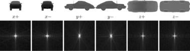
Fig. 7.2 Depth-buffer renderings. The top row shows the depth buffers of the 3D model. The bottom row shows their coefficient magnitudes of the 2D Fourier transform. Figure courtesy of [27]

After computing the Fourier coefficients, the final depth-buffer descriptor is formed as follows. First, one needs to set a parameter value k N. Then, a set of values p and q are computed, such that they hold the inequality

|p − n/2| + |q − n/2| ≤ k ≤ n/2.

The absolute values of the coefficients F (p, q) corresponds to the attributes of the final feature vector. It follows that the number of considered coefficients is k2 + k + 1. As we must repeat this process for each face of the bounding cube, the final dimensionality of the descriptor is 6(k2 + k + 1). Vranic [106] recommends setting k = 8, thus obtaining a feature vector of 438 dimensions.

Figure 7.2 shows the depth buffer renderings for a 3D model of a car. The first row of images shows the depth buffers of the 3D model. Darker pixels indicate that the distance between the view plane and the object is smaller than at brighter pixels. The second row shows coefficient magnitudes of the 2D Fourier transform of the six images.

7.3.1.3 Evaluation

The effectiveness of the depth-buffer descriptor was compared with several featurebased descriptors for 3D model retrieval [27]. The experimental evaluation showed that descriptors based on 2D projections of the 3D model can be more effective than other global descriptors. In particular, the depth-buffer descriptor got the highest average effectiveness among all descriptors, for queries in a heterogeneous 3D model dataset (Konstanz 3D Model Database). The dataset contained 1838 3D objects collected from the Internet. From the entire collection, 472 objects were used as queries and these contained a manual classification. Table 7.3 shows the results obtained in the experiments. In this case, the R-Precision measure was used in the evaluation.

An advantage of the depth-buffer technique is its low computational cost. In addition, regarding global retrieval, it is the technique with the best effectiveness. However, as can be noted, this method is not suitable to overcome problems such as partial matching and non-rigid retrieval. For more details about the evaluated techniques, we refer the reader to the original paper.

7.3.1.4 Complexity Analysis

Given a 3D object with F triangular faces, and let n be the number of bins for the depth-buffer. In addition, let k be the number of coefficients taken after the FFT. The complexity for each stage of the method is as follows:

•Construction of the depth images: O(F n2). In the worst case, each face is projected onto the entire image.

•Fast Fourier Transform: O(n2 log n).

•Linear search: O(P (k2 + k + 1)), where P is the number of descriptors stored in

the collection. The expression regarding k is because each distance computation is performed between descriptors of dimension 6(k2 + k + 1).

Therefore, the total complexity of this method is dominated by the complexity of the Fourier transform, i.e. O(n2 log n)

7.3.2 Spin Images for Object Recognition

In this section, we describe a 3D object recognition technique with support for occlusion and cluttered scenes. Originally, this work was proposed by Johnson and Hebert [56, 57] for recognizing objects in complex scenes obtained through a structured light range camera in order to be used in robotic systems. This has been recognized as pioneering work in the use of 3D shape matching for computer vision tasks

and its relative success has generated increasing interest in these kinds of techniques to support high level vision tasks. In addition, the central idea behind this technique, the spin image, is one of the pioneering local 3D shape descriptors. Broadly speaking, this technique works as follows:

•Given a set of 3D models (scans), we calculate a spin image for each vertex and store them in a huge collection of spin images.

•Given a scene, possibly cluttered and with occlusions, random vertices are selected for which spin images are computed. Thus, we compare these spin images with those previously stored and select possible correspondences.

•Finally, we need to use geometric consistency and a variation of the iterative closest point algorithm to perform correspondences validation and matching.

In order to calculate the spin images for a 3D shape, a uniform mesh is required. By uniform, we mean that distances between adjacent vertices remain close to the median of all distances. In fact, mesh resolution is defined as the median of all edge lengths from the shape. Johnson [56] proposed an efficient algorithm to control the mesh resolution which is based on mesh simplification schemes [45]. In addition, vertices have to be oriented, so each vertex must have an associated normal pointing towards the outside of the shape. We assume that a shape is uniform and each vertex is properly oriented.

To build a spin image of a vertex, we need to build a local basis defined on this vertex, so accumulating the surrounding vertices around the analyzed vertex using the local basis allows us to create a pose invariant local description. In addition, we can control how local this description is, hence the spin images can be used with large support for alignment and registration tasks and with small support for cluttered recognition.

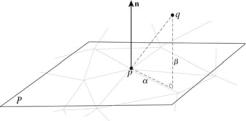
We denote an oriented point p as a pair O = (p, n) which maintains coordinate information along with the associated normal vector n. The local basis is formed by the following elements:

•The point p.

•The normal n and the line L through p parallel to n.

•The tangent plane P through p oriented perpendicularly to n.

We can represent any point q in this basis, as shown in Fig. 7.3, through two cylindrical coordinates: α, the perpendicular distance from q to the line L; and β, the signed perpendicular distance from q to the plane P. We define the spin-map SO

Fig. 7.3 Local basis for point p

as a function that projects 3D points q to the local 2D coordinates defined with the previous elements

The process of spin image formation uses the function previously defined accumulating points in the (α, β) image coordinate. This can be seen as spinning a matrix around a point’s normal and storing the occurrences of surrounding points in the respective coordinates in the matrix. Finally, the spin image looks like an occurrence histogram in the cylindrical coordinate system defined by the local basis.

In order to create a spin image, three useful parameters have to be defined

•Bin size (bin), spatial extent for the bins in the image.

•Image width (W ), number of bins in both image directions. Usually, spin images are square.

•Support angle (As ), the maximum angle between normals for contributing points.

Let A = (pA, nA) be an oriented point for which we want to build its spin image. For each oriented point B = (pB , nB ) on the shape, we use the local basis and the spin-map function to obtain the coordinate (α, β). Then, the bin corresponding to that coordinate is given by

W bin − β

i = 2

bin

(7.3)

α

j =

bin

Instead of directly accumulating the occurrence in the respective bin, the authors suggested the use of bilinear interpolation to accumulate the occurrence in neighboring positions. Therefore, bilinear weights are calculated as follows

With these weights, the image is updated as follows

I (i, j ) = I (i, j ) + (1 − a)(1 − b)

I (i, j + 1) = I (i, j + 1) + (1 − a)b

(7.5)

I (i + 1, j ) = I (i + 1, j ) + a(1 − b)

I (i + 1, j + 1) = I (i + 1, j + 1) + ab