Материал: [2.1] 3D Imaging, Analysis and Applications-Springer-Verlag London (2012)

7 3D Shape Matching for Retrieval and Recognition |
285 |
Table 7.5 Robustness results for Dense Heat Kernel Signatures. Table reproduced from Bronstein et al. [21]
Transform. |
|
Strength |
|
|
|
|
|
1 |
≤2 |
≤3 |
≤4 |
≤5 |
|
Isometry |
0.01 |
0.01 |
0.01 |
0.01 |
0.01 |
|
Topology |
0.02 |
0.02 |
0.02 |
0.02 |
0.02 |
|
Holes |
0.02 |
0.02 |
0.02 |
0.03 |
0.03 |
|
Micro holes |
0.01 |
0.01 |
0.01 |
0.01 |
0.02 |
|
Scale |
0.25 |
0.15 |
0.13 |
0.14 |
0.16 |
|
Local scale |
0.02 |
0.03 |
0.05 |
0.07 |
0.10 |
|
Sampling |
0.02 |
0.02 |
0.02 |
0.02 |
0.02 |
|
Noise |
0.03 |
0.06 |
0.09 |
0.12 |
0.15 |
|
Shot noise |
0.01 |
0.01 |
0.02 |
0.02 |
0.02 |
|
Average |
0.04 |
0.04 |
0.04 |
0.05 |
0.06 |
|
|
|
|
|
|
|
|
•Computation of spin images for each vertex: O(n2). Given a vertex, each vertex on the mesh is mapped onto its spin image.
•Find the initial set of correspondences: O(nP W 2), where P is the number of spin images in the collection. For each vertex on the query object, the cross-correlation is calculated with respect to each spin image in the collection.
•Filter the correspondences: O(n2).
•Group the correspondences: O(n2). For each correspondence, a group is computed by applying the Wgc measure.
•Find the transformation using the least squares method: O(n).
•Validation: O(n).
The total complexity is dominated by the process of finding the initial set of
correspondences. This is because P |
n, so the complexity of this method is |
O(nP W 2). |
|
7.3.3 Salient Spectral Geometric Features
In this section, we present a retrieval method based on local features extracted from the Laplace-Beltrami operator of a shape [52]. Some theoretical background is needed in order to understand the Laplace operator on manifolds and its computation. Detailed information can be found in the works by Reuter et al. [90] and Meyer et al. [77]. In addition, further relevant references can be found in Sect. 7.6.
Let f C2 be a real-valued function defined on a Riemannian manifold M. The Laplace-Beltrami operator is defined as
f = div(grad f ) |
(7.14) |
with grad f the gradient of f and div the divergence on the manifold.

286 |
B. Bustos and I. Sipiran |
If M is a domain in the Euclidean plane, the Laplace-Beltrami operator reduces to the well-known expression
f = |
∂2f |
+ |
∂2f |
(7.15) |
(∂x)2 |
(∂y)2 |
Thus, we are interested in the Helmholtz equation
f = −λf |
(7.16) |
where λ is a real scalar. This equation is important because the family of eigenvalues 0 ≤ λ0 ≤ λ1 ≤ · · · ≤ +∞ is the shape spectrum which is isometric invariant1 as it only depends on the gradient and the divergence, dependent only on the Riemannian structure of the manifold. Another important property is that the LaplaceBeltrami operator is Hermitian, so the eigenvectors vi and vj corresponding to different eigenvalues λi and λj are orthogonal:
vi · vj = vi vj = 0, i = j (7.17)
M
In addition, the i-th eigenvector defines a coefficient over the function f as fol-
lows |
|
ci = f · vi = M f vi |
(7.18) |
so the function f can be expanded as |
|
f = c1v1 + c2v2 + · · · |
(7.19) |
Given a 3D mesh, we can calculate the discrete Laplace-Beltrami operator at each vertex with the cotangent scheme proposed by Meyer et al. [77]:
|
1 |
|
|
K(pi ) = |
2Ai pj N1(pi )(cot αij + cot βij )(pi − pj ) |
(7.20) |
|
where Ai is the Voronoi region area around pi , αij and βij are the angles opposite to the arc pi pj and N1(pi ) is the set of pi ’s adjacent vertices. See Fig. 7.5 for details.
The computation of Ai , the Voronoi region around a vertex pi , must be performed as follows. We accumulate a region for each adjacent face T to pi , if T is non-obtuse we add the Voronoi region for that face by using Eq. (7.21). If T is obtuse, we add area(T)/2 if the angle of T at pi is obtuse, or area(T)/4 otherwise.
|
1 |
|
|
AT = |
|
(cot αij + cot βij ) pi − pj 2 |
(7.21) |
8 |
|||
|
|
j N1(i) |
|
1The shape spectrum of two shapes with a non-rigid transformation is approximately the same.

7 3D Shape Matching for Retrieval and Recognition |
287 |
Fig. 7.5 Neighborhood configuration around pi . The dashed lines enclose the Voronoi region used in computing the Laplace-Beltrami operator
To numerically compute the Laplace-Beltrami operator, a matrix L = {Lij } can be calculated in the following way:
|
|
|
|
|
|
cot αij +cot βij |
|
if pi is adjacent to pj |
|
|
|
|
|
ij = |
|
|
|
2Ai |
|
|
|
|
|
|
|
k |
2Ai |
|
if pi = pj |
|
||
|
|
|
|
|
|
|
|
|
|
|
|
|
|
|
|
|
|
|
|
|
|
|
|
L |
|
− |
|
cot αik +cot βkj |
|
(7.22) |
||
|
|
|
|
|
|
|||||
|
|
|
|
|
0 |
|
|
|
otherwise, |
|
|
|
|
|
|
|
|
|
|||
where p |
k are the |
|
|
|
|
|
i |
. |
|
|
|
vertices adjacent to p |
|
|
|||||||
We are interested in the eigenvalues and eigenvectors of this matrix. Thus, the
problem to be solved is: |
|
Lv = λv |
(7.23) |
However, it is clear to note that L might not be symmetric. This is to say, Lij = Lj i when Ai = Aj , which is very likely. Nevertheless, it can be represented as a generalized eigenvalue problem where L = S−1M. Then, we have:
|
|
|
|
|
Mv = λSv |
(7.24) |
||
where M = {Mij } with |
|
|
|
|
|
|
|
|
|
|
− |
cot αij +cot βij |
if pi is adjacent to pj |
|
|||
|
|
|
|
2 |
|
|
||
M |
ij = |
|
cot αik +cot βkj |
if pi = pj |
(7.25) |
|||
|
|
|
k |
2 |
|
|
||
|
|
|
|
|
|
|
|
|
|
|
|
|
|
|
|
otherwise |
|
|
|
0 |
|
|
|
|
|
|
|
|
|
|
|
|
|
|
|
|
|
|
|
|
|
|
|
|
|
|
|
|
|
|
|
|
|
and S = {Sij } with |
|
|
|
|
|
|
|
|
|
|
|
|
S |
Ai |
if i = j |
(7.26) |
|
|
|
|
|
|
ij = 0 |
otherwise |
|
|
The solution to this problem ensures that the eigenvalues and eigenvectors are real. In addition, two eigenvectors vi and vj corresponding to different eigenvalues λi and λj are orthogonal with respect to the S dot-product:
vi · vj = viT Svj = 0, i = j |
(7.27) |
288 |
B. Bustos and I. Sipiran |
The shape spectrum is the set of eigenvalues {λ0, λ1, λ2, . . . , λn−1}. If the shape is closed, λ0 = 0.
7.3.3.1 Feature Points Detection
Recalling the problem of geometric reconstruction, we have the vertices set P = [X Y Z] where X, Y and Z are column vectors containing the values of their coordinates. In addition, we define a coefficient matrix C = PT SV where S is the diagonal matrix as stated before and V is a N × N matrix with each column being an eigenvector. The eigenvectors are ordered according to their associated eigenvalues, from low to high. Thus, we can obtain the vertices set with:
P = VCT |
(7.28) |
We introduce the matrix notation A1−p,1−q as the submatrix with rows from 1 to p and columns from 1 to q. Using this notation, we can express the reconstruction problem using the first k eigenvectors:
P(k) = V1−n,1−k CT− − (7.29)
1 3,1 k
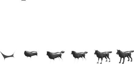
As can be noted, P(k) has the same size as P, but the vertex position is dependent on k. We can use P(k) with the original connections for evaluating the information gained with different k values (see Fig. 7.6). The authors defined a geometric energy at a vertex i corresponding to the kth eigenvector as:
E(i, k) = V (i, k) × C1−3,k |
2 |
(7.30) |
|
|
|
The authors evaluated E in order to detect interest points. A vertex pi is selected if E(i, k) > E(j, h) for all vertex pj adjacent to pi in the original mesh and for all
h [k − 1, k, k + 1]. Furthermore, each selected vertex has an associated scale fac-
√
tor sf = 1/ λk . An important fact to be considered here is that the same vertex can be selected with different associated scale factors. The authors proposed to evaluate only the first 100 eigenvectors because they claimed that more eigenvectors do not contribute significant spatial and spectral energy. The first eigenvectors are associated to the coarse structure of the mesh and later eigenvectors are associated with the detailed geometry. Thus the last eigenvectors could be associated with noise. In this respect, the number of vertices could give us an insight concerning how many eigenvectors might be used, because the maximum number of eigenvectors equals the number of vertices.
Fig. 7.6 Effect of reconstructing P(k) using k = 5, 20, 50, 100, 300, and 1000, respectively over a shape with 8000+ vertices
7 3D Shape Matching for Retrieval and Recognition |
289 |
As the eigenvalues are increasing and the first eigenvectors are related to large scales, taking the scale as previously defined seems to be a good approximation, although the relation between the eigenvalues and the real spatial scale of the interest points is not clear.
7.3.3.2 Local Descriptors
To create local descriptors associated with each interest point, the Laplace-Beltrami operator can be used in a straightforward way. The process starts by selecting a patch based on the scale information of each vertex. Given an interest point, pi , we select a mesh patch formed by the vertices with geodesic distance from pi not exceeding the radius r × sf(pi ) (in the experiments, r was 1.7). The extracted patch is an open boundary surface, so that we need to attach another patch in order to apply the Laplace-Beltrami operator with successful results. The authors proposed to attach the same patch but in the opposite direction. Once we have a closed local surface, we apply the aforementioned method in order to obtain the spectrum.
The local descriptor is defined as the set {λ1, λ2, . . . , λm} for some value m. For similarity comparison, the spectrum must be normalized in order to allow scale invariance. This can be done by dividing each element in the local descriptor with the first eigenvalue λ1.
7.3.3.3 Shape Matching
From the preceding stages, each mesh is represented as a set of descriptors, so now we are interested in comparing two objects based on this information. Given two descriptor sets P = {pi } and P = {pi }, the problem is to find a transformation function φ such that:
i |
) |
= |
i |
(7.31) |
φ (p |
|
p |
Thus, the similarity function is defined as:
Sim(φ) = Sims (φ) + Simp (φ) |
(7.32) |
Sims (φ) refers to the feature-to-feature comparison and Simp (φ) to the cluster- to-cluster similarity. The feature-to-feature similarity is defined as follows:
|
Sims (φ) = ωs |
|
|
|
|
|||
|
C i, i |
|
(7.33) |
|||||
|
|
|
|
φ (i)=i |
|
|
|
|
where |
|
= |
− |
2σs2 |
|
|
|
|
|
|
|
|
|||||
C |
i, i |
|
exp |
|
f (i) − f (i ) 2 |
(7.34) |
||
|
|
|
||||||
where f (.) is the local descriptor of a point and σs |
is a constant. |
|||||||