Материал: [2.1] 3D Imaging, Analysis and Applications-Springer-Verlag London (2012)

290 |
B. Bustos and I. Sipiran |
In addition, the cluster-to-cluster similarity is defined as:
|
|
|
Simp (φ) = ωp |
|
|
|
|
|
|
|
H |
i, j, i , j |
|
|
|
||||||||
|
|
|
|
|
|
|
|
|
|
|
|
|
i ,φ (j ) |
= |
j |
|
|
|
|
|
|
||
|
|
|
|
|
|
|
|
|
|
φ (i)= |
|
|
|
|
|
||||||||
where |
|
|
|
|
|
|
|
|
|
|
|
|
|
|
|
|
|
|
|
|
|
|
|
H i, j, i |
, j |
|
|
= |
exp |
|
−(dpg (i, j, i , j ) + βdps (i, j, i , j |
))2 |
|
||||||||||||||
|
|
|
|
|
|||||||||||||||||||
|
|
|
|
|
|
|
|
|
|
|
|
2σp2 |
|
|
|
|
|
||||||
where |
|
|
|
|
|
|
|
|
|
|
|
|
|
|
|
|
|
|
|
|
|
|
|
|
|
|
|
dpg i, j, i , j |
|
|
= |
|
g(i, j ) |
− |
g(i , j ) |
|
|
|
|
|
|||||||
|
|
|
|
sf(i) |
|
sf(i ) |
|
|
|
|
|||||||||||||
|
|
|
|
|
|
|
|
|
|
|
|
|
|
|
|
|
|
|
|
|
|
|
|
and |
|
|
|
|
|
|
|
|
|
|
|
|
|
|
|
|
|
|
|
|
|
|
|
|
|
|
|
|
|
|
|
|
|
|
|
|
|
|
|
|
|
|
|
|
|
|
|
|
dps |
i, j, i , j |
|
= |
|
|
|
|
sf(j ) |
|
|
sf(j |
) |
|
|
||||||||
|
|
log sf(i) − log sf(i ) |
|
||||||||||||||||||||
|
|
|
|
|
|
|
|
|
|
|
|
|
|
|
|
|
|
|
|
|
|
||
|
|
|
|
|
|
|
|
|
|
|
|
|
|
|
|
|
|
|
|
|
|
|
|
|
|
|
|
|
|
|
|
|
|
|
|
|
|
|
|
|
|
|
|
|
|
|
|
(7.35)
(7.36)
(7.37)
(7.38)
where g(·, ·) is the geodesic distance between two vertices, sf(·) is the vertex scale factor calculated in the feature detection stage and σp is a constant.
In order to solve the matching problem using the defined similarity measure, we need to define an indicator variable
|
x |
i, i |
|
|
|
|
1 |
if φ (i) = i exists |
|
|
(7.39) |
|
|
|
|
|
= |
0 |
otherwise |
|
|
|
|||
|
|
|
|
|
|
|
||||||
We can reformulate the similarity measure using the indicator variable as |
||||||||||||
|
|
|
|
|
|
+ ωs |
|
|
|
|
|
|
Sim(x) = ωp |
C i, i |
x i, i |
|
|
H i, j, i , j |
x i, i |
x j, j |
(7.40) |
||||
i,i |
|
|
|
|
|
|
|
i,j,i ,j |
|
|
|
|
subject to i x(i, i ) ≤ 1 and |
|
|
|
i x(i, i ) ≤ 1. These expressions impose the con- |
||||||||
each point in the first descriptor set has at most one correspondence in |
||||||||||||
straint that |
|
|
|
|
|
|
|
|
|
|
||
the second descriptor set. To numerically solve this problem, we can use Integer Quadratic Programming (IQP) as follows
max |
Sim(x) = x |
T H |
x + |
CT |
x subject to |
A |
x ≤ b |
(7.41) |
x |
|
|
|
We now describe some details for implementation. Let N be the number of descriptors in P and M be the number of descriptors in P . After calculating the matrix C, we have to convert it in a column vector concatenating each column in the matrix so that the dimension of C is N M × 1. Note that the size of H is N M × N M because we need to calculate H(i, j, i , j ) between each pair of descriptor from P with each pair from P . With respect to the constraints on the number of correspondences, these have to be located in the matrix A and a vector b. The geodesic distances can be approximated using a shortest path algorithm on the mesh, however another clever algorithm can also be used such as the fast marching method
7 3D Shape Matching for Retrieval and Recognition |
291 |
proposed by Kimmel and Sethian [62]. In order to solve the aforementioned optimization problem, there are several alternatives such as the MATLAB’s optimization toolbox or the CGAL library [2].
In summary, the method can be described as follows.
1.Solving the Laplace-Beltrami eigenproblem: We need to compute the eigenvectors and eigenvalues of the Laplace-Beltrami operator for each shape in the dataset.
2.Feature points detection: Computing the geometric energy given in Eq. (7.30), it is possible to select the interest points along with their scales.
3.Construction of local descriptors: For each interest point, the method extracts a local patch over which the Laplace-Beltrami operator is calculated. A few normalized eigenvalues of this operator are considered as a local descriptor.
4.Matching: The problem of multi-feature matching is considered as an integer quadratic programming problem, as given in Eq. (7.41).
7.3.3.4 Evaluation
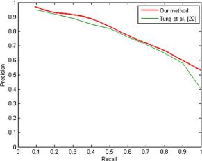
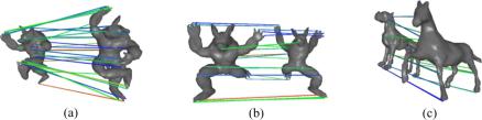
In the original work by Hu and Hua [52], several tests were accomplished for shape correspondence and shape retrieval over the SHREC’07 3D shape database available at http://www.aimatshape.net/event/SHREC. The authors proposed to extract 10 shapes from each category of the dataset. Figure 7.7 shows the precision-recall plot for the presented approach compared to the best technique in the SHREC’07 watertight retrieval contest. In addition, Fig. 7.8 present an example of matching between shapes in the same category and between shapes in different categories.
From the results, it is important to note that the method performs well on nonrigid transformations. In fact, it outperforms the best technique in the SHREC’2007
Fig. 7.7 Precision-recall plot for the salient spectral features approach. Figure courtesy of [52]
292 |
B. Bustos and I. Sipiran |
Fig. 7.8 (a, b) Matching with shapes from the same category. (c) Matching between shapes from different categories. Figure courtesy of [52]
dataset. Also, an important aspect of this technique is that it delivers a set of correspondences between salient points, in addition to the matching score. It is valuable because two problems (matching and correspondences) can be addressed with the same approach.
7.3.3.5 Complexity Analysis
Let S be a 3D object with n vertices. In the following, we list the computational complexity associated with the various stages of the presented approach.
•Compute the Laplacian matrix: O(n2).
•Compute eigenvalues and eigenvectors of the Laplacian matrix: O(n3).
•Interest point detection: O(nk), if k eigenvectors are chosen.
•Interest point description: O(mq3), where m is the number of detected interest points and q is the number of vertices in the patch associated to each interest point.
•Matching: Let suppose two objects P and Q with N and M interest points, respectively. The computational complexities of each step of the matching are:
–Computation of matrix C: O(N M).
–Computation of matrix H: O(N 3M2 log N ). The matrix H corresponds with all the possible combinations of correspondence pairs. For each pair, the computation of the geodesic distance takes O(N log N ).
–Solve the IQP problem: O(N 2M2).
The total complexity of this method is dominated by the calculation of the matrix H, due to the computation of the geodesic distances between interest points. Therefore, the complexity of this method is O(N 3M2 log N ).
7.3.4 Heat Kernel Signatures
We observed in the previous approach the importance and applicability of the Laplace-Beltrami operator and its spectrum in shape description tasks. In this section, we describe the application of heat kernel signatures which are based on the
7 3D Shape Matching for Retrieval and Recognition |
293 |
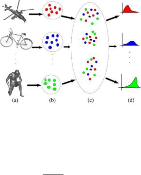
Fig. 7.9 Process to obtain a descriptor for a shape using the heat kernel signatures and bag of features. (a) Input shape, (b) local descriptors (heat kernel signatures) are extracted, (c) clustering of descriptor space (black stars are centroids of resulting clusters), and (d) Vector quantization, using local descriptors and clusters, results in shape descriptors
intimate relation between the heat diffusion process and the Laplace-Beltrami operator. In addition, the presented technique utilizes a widely-used approach for describing information entities based on their components and frequencies known as Bag-of-Features [83]. Figure 7.9 summarizes the approach.
The heat diffusion process over a compact manifold S, possibly with boundary, is governed by the heat equation
Su(x, t ) = − |
∂u(x, t ) |
(7.42) |
∂t |
where S is the Laplace-Beltrami operator of S and u(., t ) is the heat distribution over S over time t .
The fundamental solution of Eq. (7.42) is Kt (x, y) called the heat kernel. This represents a solution with a point heat source at x and can be considered as the amount of heat transferred from x to y after time t . For compact manifolds, the heat kernel can be expressed using the eigenvalues and eigenvectors of the LaplaceBeltrami operator as follows:
∞ |
|
|
|
Kt (x, y) = exp(−λi t )vi (x)vi (y) |
(7.43) |
i=0
where λi is the i-th eigenvalue and vi (·) is the i-th eigenvector’s entry corresponding to a given point.
Sun et al. [97] formally proved that the heat kernel is an isometric invariant, informative (redundant information exists), multi-scale, and stable against perturbations of the surface. In addition, restricting the heat kernel to the temporal domain and fixing the spatial variables, we can obtain a representation for each point on the manifold:
∞ |
|
|
|
Kt (x, x) = exp(−λi t )vi (x)2 |
(7.44) |
i=0
294 |
B. Bustos and I. Sipiran |
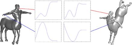
Fig. 7.10 Heat kernel signatures calculated on two isometric shapes. At top, signatures in corresponding points look very similar. At bottom, signatures in different points on the mesh differ
In Fig. 7.10, we show heat kernel signatures for two isometric shapes. Given a shape S, we need to calculate the heat kernel signature for a point on S. In practice, the heat kernel signature p(x) of a point x S is an n-dimensional descriptor vector with each bin corresponding to some value of t :
|
i (x) = |
|
α |
− |
t0 |
|
p(x) = |
|
p1(x), . . . , pn(x) |
(7.45) |
|||
p |
|
c(x)K i |
1 |
(x, x) |
(7.46) |
|
where c(x) must be selected in order to have p(x) 2 = 1. Note that we need to restrict the number of eigenvalues and eigenvectors to be considered in Eq. (7.44). As a result, we obtain a descriptor for each vertex on the mesh.
Once we have computed the descriptors for each shape in the database, these must be grouped in a huge collection of local descriptors which will be called the descriptor space. Next, it is necessary to quantize the n-dimensional descriptors space. The idea is to find a point set in the descriptor space in order to better cluster the whole descriptor set. Unsupervised techniques from machine learning field can be used such as k-means and its variants [38]. In order to make this section relatively self-contained, we briefly describe k-means clustering in the descriptor space.
Let D be the huge set of n-dimensional descriptors and k be the number of clusters we want to find. The algorithm can be summarized as follows:
1.Initial centroids selection: Select k points in the n-dimensional space. This step can be performed in different ways, for instance, selecting random points in the n-dimensional space, selecting random descriptors from D, or using in-
formation about the distribution of descriptors in D, just to name a few. Let M = {m1, . . . , mk } be the set of selected centroids.
2.Cluster assignment: Assign each descriptor d in D to the closest cluster Ci
Ci = d D : d − mi ≤ d − mj , j = 1 . . . k |
(7.47) |