Материал: [2.1] 3D Imaging, Analysis and Applications-Springer-Verlag London (2012)

dark regions such as the eyebrows and facial hair are usually not acquired. Moreover, for laser-based projection, power cannot be increased to acquire dark regions of the face due to eye-safety reasons.

Thus the only option is to fill the missing regions using an interpolation technique such as nearest neighbor, linear or polynomial. For small holes, linear interpolation gives reasonable results however, bicubic interpolation has shown to give better results [64]. Alternatively one can use implicit surface representations for interpolation, such as those provided by radial basis functions [72].

For larger size holes, symmetry or PCA based approaches can be used, although these require a localized symmetry plane and a full 6-DOF rigid alignment respectively, and hence would have to be moved further downstream in the processing pipeline. Alternatively, a model-based approach can be used to morph a model until it gives the best fit to the data points [95]. This approach learns the 3D face space offline and requires a significantly large training data in order to generalize to unseen faces. However, it may be very useful if the face being scanned was previously seen and obviously this is a common scenario in 3D face recognition.

For better generalization to unseen faces, an anthropometrically correct [32] annotated face model (AFM) [51] is used. The AFM is based on an average 3D face constructed using statistical data and the anthropometric landmarks are associated with its vertices. The AFM is then fitted to the raw data from the scanner using a deformable model framework. Blanz et al. [12] also used a morphable model to fit the 3D scan, filling up missing regions in addition to other preprocessing steps, in a unified framework.

8.5.4 Removal of Noise

For face scans acquired by laser scanners, noise can be attributed to optical components such as the lens and the mirror, or mechanical components which drive the mirror, or the CCD itself. Scanning and imaging conditions such as ambient light, laser intensity, surface orientation, texture, and distance from the scanner can also affect the noise levels in the scanner. Sun et al. [89] give a detailed analysis of noise in the Minolta Vivid scanner and noise in active sensors is discussed in detail in Chap. 3 of this book.

We have already mentioned the median filter as a mechanism for spike (impulsive noise) removal. More difficult is the removal of surface noise, which is less differentiated from the underlying object geometry, without removing fine surface detail or generally distorting the underlying shape, for example, from volumetric shrinkage. Clearly, there is a tradeoff to be made and an optimal level of filtering is sought in order to give the best recognition performance. Removal of surface noise is particularly important as a preprocessing step in some methods of extraction of the differential properties of the surface, such as normals and curvatures.

If the 3D data is in range image or depth map form, there are many methods available from the standard 2D image filtering domain, such as convolution with

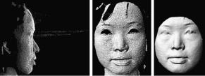
Fig. 8.6 From left to right. A 3D capture of a face with spikes in the point cloud. Shaded view with holes and noise. Final preprocessed 3D data after cropping, removal of spikes, hole filling and noise removal. Figure courtesy of [64]

Gaussian filters. Many of these methods have been adapted so that they can be applied to 3D meshes. One example of this is Bilateral Mesh Denoising [35], which is based on shifting mesh vertices along their normal directions.

Figure 8.6 shows a face scan with spikes, holes and noise before and after preprocessing.

8.5.5 Fiducial Point Localization and Pose Correction

The pose of different subjects or the same subject can vary between scans even when they are cooperative. Therefore, pose correction is a necessary preprocessing step for holistic approaches that require normalized resampling of the facial surface in order to generate a feature vector. (Such feature vectors are often subsequently mapped into a subspace; for example, in PCA and LDA-based methods described later.) This may also be necessary for other algorithms which rely on features that are not inherently pose-invariant.

A common approach to pose correction uses fiducial points on the 3D face. Three points are necessary to normalize the pose to a canonical form. Often these points are manually identified, however, automatic detection of such points is desirable particularly for online verification and identification processes.

The shape index, derived from principle curvatures, has been used to automatically detect the inside eye corners and the nose tip for facial pose correction [59]. Although, a minimum of three fiducial points are sufficient to correct the pose, it has proved a challenging research problem to detect these points, where all three are identified correctly and localized with high repeatability. This problem is more difficult in the presence of varying facial expression, which can change the local shape around a point. Worse still, as pose changes, one of the three fiducial points selected may become occluded. For example, the nose bridge occludes an inner eye corner as the head is turned from frontal view towards a profile view. To counter this, some approaches have attempted to extract a large number of fiducial points so that three or more are always visible [24].

In addition to a shape scan, most 3D cameras capture a registered color-texture map of the face (i.e. a standard 2D image, where the color associated with each 3D

can be measured in absolute units (e.g. millimeters). Thus scanning the same face from near or far will only alter the spatial sampling rate and the measured distance between landmarks should vary very little, at least in scans of reasonable quality and resolution.

However, many face recognition algorithms require the face surface, or parts of the face surface, to be sampled in a uniform fashion, which requires some form of spatial sampling normalization or spatial resampling via an interpolation process. Basic interpolation processes usually involve some weighted average of neighbors, while more sophisticated schemes employ various forms of implicit or explicit surface fitting.

Assuming that we have normalized the pose of the face (or facial part), we can place a standard 2D resampling grid in the x, y plane (for example, it could be centered on the nose-tip) and resample the facial surface depth orthogonally to generate a resampled depth map. In many face recognition schemes, a standard size feature vector needs to be created and the standard resampling grid of size p × q = m creates this. For example, in [64], all 3D faces were sampled on a uniform x, y grid of 161 × 161 where the planar distance between adjacent pixels was 1 mm. Although the sampling rate was uniform in this case, subjects had a different number of points sampled on their faces, because of their different facial sizes. The resampling scheme employed cubic interpolation. In another approach, Pears et al. [72] used RBFs as implicit surface representations in order to resample 3D face scans.

An alternative way of resampling is to identify three non-collinear fiducial points on each scan and resample it such that the number of sample points between the fiducial points is constant. However, in doing this, we are discarding information contained within the absolute scale of the face, which often is useful for subject discrimination.

8.5.7 Feature Extraction on Facial Surfaces

Depth maps may not be the ideal representations for 3D face recognition because they are quite sensitive to pose. Although the pose of 3D faces can be normalized with better accuracy compared to 2D images, the normalization is never perfect. For this reason it is usually preferable to extract features that are less sensitive to pose before applying holistic approaches. The choice of features extracted is crucial to the system performance and is often a trade-off between invariance properties and the richness of information required for discrimination. Example ‘features’ include the raw depth values themselves, normals, curvatures, spin images [49], 3D adaptations of the Scale-Invariant Feature Transform (SIFT) descriptor [57] and many others. More detail on features can be found in Chaps. 5 and 7.

8.5.8 Classifiers for 3D Face Matching

In the large array of published 3D face recognition work, all of the well-known classification schemes have been applied by various researchers. These include k-nearest neighbors (k-NN) in various subspaces, such as those derived from PCA and LDA, neural nets, Support Vector Machines (SVM), Adaboost and many others. The choice (type, complexity) of classifier employed is related to the separation of subjects (classes) within their feature space. Good face recognition performance depends on choosing a classifier that fits the separation of the training data well without overfitting and hence generalizes well to unseen 3D face scans, either within testing or in a live operational system.

Pattern classification is a huge subject in its own right and we can only detail a selection of the possible techniques in this chapter. We refer the reader to the many excellent texts on the subject, for example [10, 28].

8.6 ICP-Based 3D Face Recognition

In this section and the following three sections, we will present a set of wellestablished approaches to 3D face recognition, with a more tutorial style of presentation. The aim is to give the reader a solid grounding before going on to more modern and more advanced techniques that have better performance. We will highlight the strengths and limitations of each technique and present clear implementation details.

One of the earliest algorithms employed for matching surfaces is the iterative closest points (ICP) algorithm [9], which aims to iteratively minimize the mean square error between two point sets. In brief, ICP has three basic operations is its iteration loop, as follows.

1.Find pairs of closest points between two point clouds (i.e. probe and gallery face scans).

2.Use these putative correspondences to determine a rigid 6-DOF Euclidean transformation that moves one point cloud closer to the other.

3.Apply the rigid transformation to the appropriate point cloud.

The procedure is repeated until the change in mean square error associated with the correspondences falls below some threshold, or the maximum number of iterations is reached. In the context of 3D face recognition, the remaining mean square error then can be used as a matching metric.

Due to its simplicity, ICP has been popular for rigid surface registration and 3D object recognition and many variants and extensions of ICP have been proposed in the literature [77]. Readers interested in a detailed description of ICP variants are referred to Chap. 6 of this book, which discusses ICP extensively in the context of surface registration.

Here, we will give a presentation in the context of 3D face recognition. Surface registration and matching are similar procedures except that, in the latter case, we