Материал: [2.1] 3D Imaging, Analysis and Applications-Springer-Verlag London (2012)

8.4 3D Face Recognition Evaluation

The evaluation of a 3D face recognition system depends on the application that it is intended for. In general, a face recognition system operates in either a verification application, which requires one-to-one matching, or an identification application, which requires one-to-many matching. We discuss each of these in turn in the following subsections.

8.4.1 Face Verification

In a verification application, the face recognition system must supply a binary accept or reject decision, as a response to the subject’s claimed identity, associated with one of a stored set of gallery scans. It does this by generating a match score between the captured 3D data (the probe or query) and the gallery data of the subject’s claimed identity. Often this is implemented as a distance metric between feature vectors, such as the Euclidean distance, cosine distance or Mahalanobis distance (in the case of multiple images of the same person in the gallery). A low score on the distance metric indicates a close match and application of a suitable threshold generates the accept/reject decision. Verification systems are mainly used by authorized individuals, who want to gain their rightful access to a building or computer system. Consequently, they will be cooperative when adopting a neutral expression and frontal pose at favorable distance from the camera. For cooperative scenarios, datasets such as FRGC v2 provide suitable training and validation datasets to perform verification tests.

In order to evaluate a verification system, a large number of verification tests need to be performed, where the subject’s identity associated with the test 3D capture is known, so that it can be established whether the accept/reject decision was correct. This identity can be extracted from the filename of a 3D face capture within a dataset by means of a unique subject identifier.

A key point is that the accept/reject decision is threshold dependent and it is desirable to explore the system performance over a wide range of such thresholds. Given that a set of 3D face scans is available, all with known identities, and there are at least two scans of each subject, we now describe a way of implementing this. Every image in the set is compared with every other, excluding itself, and a match score is formed. Two lists are then formed, one containing matches of the same subject identity and the other containing matches of different subjects. We then vary the threshold from zero so that all decisions are reject, to the maximum score value, so that all decisions are accept. For each threshold value, we examine the two lists and count the number of reject decisions from the same identity (SI) list to form a false rejection rate (FRR) as a percentage of the SI list size and we count the number of accept decisions in the different identity (DI) list to form a false acceptance rate (FAR) as a percentage of the DI list size. Ideally both FAR and FRR would be both zero and this describes a perfect system performance. However, in reality, verification systems are not perfect and both false accepts and false rejects exist. False

accepts can be reduced by decreasing the threshold but this increases false rejects and vice-versa. A receiver operating characteristic or ROC curve, as defined in biometric verification tests, is a plot of FRR against FAR for all thresholds, thus giving a visualization of the tradeoff between these two performance metrics. Depending on the dataset size and the number of scans per person, the SI and DI list sizes can be very different, with DI usually much larger than SI. This has the implication that values on the FRR axis are noisier than on the FAR axis.

In order to measure system performance using a ROC curve we can use the concept of an equal error rate (EER), where FAR = FRR, and a lower value indicates a better performance for a given face verification system. Given that a false accept is often a worse decision with a higher penalty than a false reject, it is common practise to set a suitably low FAR and then performance is indicated by either the FRR, the lower the better, or the true accept rate, TAR = 1 − FRR, the higher the better. TAR is commonly known as the verification rate and is often expressed as a percentage. In FRGC benchmark verification tests this FAR is set at 0.001 (0.1 %).

At the time of writing, high performance 3D face recognition systems are reporting verification rates that typically range from around 96.5 % to 98.5 % (to the nearest half percent) at 0.1 % FAR on the full FRGC v2 dataset [51, 64, 76]. This is a significant performance improvement of around 20 % on PCA-based baseline results [71]. It is reasonable to assume that, in many verification scenarios, the subject will be cooperating with a neutral expression. Verification rates for probes with neutral expressions only range from around 98.5 % to 99.5 % [51, 64] at 0.1 % FAR.

8.4.2 Face Identification

In face identification, the probe (query) 3D capture is matched to a stored gallery of 3D captures (‘models’), with known identifier labels, and a set of matching scores is generated. Thus identification requires a one-to-many match process in contrast to verification’s one-to-one match. The match with the highest match score (or, equivalently, lowest distance metric) provides the identity of the probe. If the closest match is not close enough by application of some threshold, the system may return a null response, indicating that the probe does not match to any subject in the gallery. This is a more difficult problem than verification, since, if there are 1000 subjects in the gallery, the system has to provide the correct response in 1001 possible responses (including the null response).

In order to test how good a 3D face recognition system is at identification, a large number of identification tests are performed, with no 3D model being compared to itself, and we determine the percentage of correct identifications. This gives the rank-1 identification rate, which means that the match is taken as the best (rank-1) score achieved when matching to the gallery. However, we can imagine real-world identification scenarios where the rank-1 identification test is too severe and where we may be interested in a wider performance metric. One such scenario is the watch list, where 3D models of a small number of known criminals may be stored in the

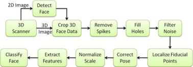
Fig. 8.5 Block diagram showing typical processing steps in a 3D face recognition system. There are several possible reorderings of this pipeline, depending on the input data quality and the performance priorities of the application

gallery, along with a larger set of the general public. If a probe matches reasonably well to any one of these criminal identities, such that the match score is ranked in the top ten, then this can trigger an alarm for a manual inspection of the probe image and top 10 gallery matches. In this case the rank-10 identification rate is important.

In practice, curves are generated by recording the rank of the correct match and then counting the percentage of identifications that are less than or equal to r , where r is the allowable rank. The allowable rank starts at 1 and is incremented until 100 % recognition is attained for some r , or the graph may be terminated before then, for example r = 100. Plotting such a Cumulative Match Curve (CMC) of percentage identification against rank allows us to compare systems at a range of possible operating points, although rank-1 identification is the most important of these.

At the time of writing, high performance 3D face recognition systems are reporting rank-1 identification rates that typically range from around 96 % to 98.5 % [51, 64, 76] on the FRGC v2 3D face dataset. We note that the FRGC v2 3D face dataset does not contain significant pose variations and performance of identification systems may fall as more challenging large scale datasets are developed that do contain such variations.

8.5 Processing Stages in 3D Face Recognition

When developing a 3D face recognition system, one has to understand what information is provided from the camera or from the dataset, what format it is presented in and what imperfections are likely to exist. The raw data obtained from even the most accurate scanners is imperfect as it contains spikes, holes and noise. Preprocessing stages are usually tailored to the form and quality of this raw data. Often, the face scans must be normalized with respect to pose (e.g. holistic approaches) and spatial sampling before extracting features for 3D face recognition. Although the 3D face processing pipeline shown in Fig. 8.5 is typical, many variations on this exist;

in particular, there are some possible reorderings and not all of the preprocessing and pose normalization stages are always necessary. With this understanding, we discuss all of the stages of the pipeline in the following subsections.

8.5.1 Face Detection and Segmentation

Images acquired with a 3D sensor usually contain a larger area than just the face area and it is often desirable to segment and crop this extraneous data as early as possible in the processing pipeline in order to speed up processing in the downstream sections of the pipeline. This face detection and cropping process, which yields 3D face segmentation, can be done on the basis of the camera’s 3D range data, 2D texture image or a combination of both.

In the case of 2D images, face detection is a mature field (particularly for frontal poses) and popular approaches include skin detection, face templates, eigenfaces, neural networks, support vector machines and hidden Markov models. A survey of face detection in images is given by Yang et al. [92]. A seminal approach for realtime face detection by Viola and Jones [88] is based on Haar wavelets and adaptive boosting (Adaboost) and is part of the Open Computer Vision (OpenCV) library.

However, some face recognition systems prefer not to rely on the existence of a 2D texture channel in the 3D camera data and crop the face on the basis of 3D information only. Also use of 3D information is sometimes preferred for a more accurate localization of the face. If some pose assumptions are made, it is possible to apply some very basic techniques. For example, one could take the upper most vertex (largest y value), assume that this is near to the top of the head and crop a sufficient distance downwards from this point to include the largest faces likely to be encountered. Note that this can fail if the upper most vertex is on a hat, other head accessory, or some types of hair style. Alternatively, for co-operative subjects in frontal poses, one can make the assumption that the nose tip is the closest point to the camera and crop a spherical region around this point to segment the facial area. However, the chin, forehead or hair is occasionally closer. Thus, particularly in the presence of depth spikes, this kind of approach can fail and it may be better to move the cropping process further down the processing pipeline so that it is after a spike filtering stage.

If the system’s computational power is such that it is acceptable to move cropping even further down the pipeline, more sophisticated cropping approaches can be applied, which could be based on facial feature localization and some of the techniques described earlier for 2D face detection. The nose is perhaps the most prominent feature that has been used alone [64], or in combination with the inner eye corners, for face region segmentation [22]. The latter approach uses the principal curvatures to detect the nose and eyes. The candidate triplet is then used by a PCA-based classifier for face detection.

8.5.2 Removal of Spikes

Spikes are caused mainly by specular regions. In the case of faces, the eyes, nose tip and teeth are three main regions where spikes are likely to occur. The eye lens sometimes forms a real image in front of the face causing a positive spike. Similarly, the specular reflection from the eye forms an image of the laser behind the eye causing a negative spike. Shiny teeth seem to be bulging out in 3D scans and a small spike can sometimes form on top of the nose tip. Glossy facial makeup or oily skin can also cause spikes at other regions of the face. In medical applications such as craniofacial anthropometry, the face is powdered to make its surface Lambertian and the teeth are painted before scanning. Some scanners like the Swiss Ranger [84] also gives a confidence map along with the range and grayscale image. Removing points with low confidence will generally remove spikes but will result in larger regions of missing data as points that are not spikes may also be removed. Spike detection works on the principle that surfaces, and faces in particular, are generally smooth.

One simple approach to filtering spikes is to examine a small neighborhood for each point in the mesh or range image and replace its depth (Z-coordinate value) by the median of this small neighborhood. This is a standard median filter which, although effective, can attenuate fine surface detail. Another approach is to threshold the absolute difference between the point’s depth and the median of the depths of its neighbors. Only if the threshold is exceeded is the point’s depth replaced with the median, or deleted to be filled later by a more sophisticated scheme. These approaches work well in high resolution data, but in sufficiently low resolution data, problems may occur when the facial surface is steep relative to the viewing angle, such as the sides of the nose in frontal views. In this case, we can detect spikes relative to the local surface orientation, but this requires that surface normals are computed, which are corrupted by the spikes. It is possible to adopt an iterative procedure where surface normals are computed and spikes removed in cycles, yielding a clean, uncorrupted set of surface normals even for relatively low resolution data [72]. Although this works well for training data, where processing time is noncritical, it may be too computationally expensive for live test data.

8.5.3 Filling of Holes and Missing Data

In addition to the holes resulting from spike removal, the 3D data contains many other missing points due to occlusions, such as the nose occluding the cheek when, for example, the head pose is sufficiently rotated (in yaw angle) relative to the 3D camera. Obviously, such areas of the scene that are not visible to either the camera or the projected light can not be acquired. Similarly, dark regions which do not reflect sufficient projected light are not sensed by the 3D camera. Both can cause large regions of missing data, which are often referred to as missing parts.

In the case of cooperative subject applications (e.g. a typical verification application) frontal face images are acquired and occlusion is not a major issue. However,