Материал: [2.1] 3D Imaging, Analysis and Applications-Springer-Verlag London (2012)

8 3D Face Recognition |
341 |
leading diagonal allowing a suitable number of eigenvectors to be selected for the subspace, as in step 5 of the previous subsection.
8.7.3 PCA Testing
Once the above PCA training phase is completed, it is straightforward to implement a simple nearest neighbor face identification scheme, within the reduced k-dimensional space. We can also threshold a suitable distance metric to implement a face verification scheme.
Each test or probe face, xp , must undergo the same transformations as the training faces, namely subtraction of the training data mean and projection into the subspace:
x˜ pT = (xp − x¯ )T Vk . |
(8.21) |
Euclidean distance and cosine distance are common metrics used to find the nearest neighbor in the gallery. Given some probe face, x˜ p , and some gallery face, x˜ g , both of which have been projected into the PCA-derived subspace, the Euclidean distance between them is given as:
de (xp , xg ) |
xp |
xg |
= |
|
(xp |
xg )T (xp |
xg ) |
˜ ˜ |
= ˜ |
− ˜ |
|
˜ |
− ˜ ˜ |
− ˜ |
and the cosine distance is given as:
x˜ T x˜ g
dc (x˜ p , x˜ g ) = 1 − p .
x˜ p · x˜ g
(8.22)
(8.23)
In both cases, a small value of the metric (preferably close to zero) indicates a good match. In testing of a PCA-based 3D face recognition system Heseltine et al. [44] found that, usually the Euclidean distance outperformed the cosine distance, but the difference between the two metrics depended on the surface feature type (depth, curvature or gradient) and in a minority of cases, the cosine distance gave a marginally better performance.
The distance metrics described above don’t take any account of how the training data is spread along the different axes of the PCA-derived subspace. The Mahalanobis distance normalizes the spread along each axis, by dividing by its associated variance to give:
dm(xp , xg ) |
|
|
|
|
|
|
|
(8.24) |
= |
(xp |
xg )T D−1 |
(xp |
xg ). |
||||
˜ ˜ |
|
˜ |
− ˜ |
˜ |
− ˜ |
|
||
This expresses the distance in units of standard deviation. Note that the inverse of D is fast to compute due to its diagonal structure. Equivalently, we can whiten the training and test data, by premultiplying all feature vectors by D− 12 , which maps the covariance of the training data to the identity matrix, and then Eq. (8.22) for the Euclidean distance metric can be used in this new space. Similarly, we can use the cosine distance metric in the whitened feature space. Heseltine et al. [44] found that
342 |
A. Mian and N. Pears |
using information in D generally improved performance in their PCA-based 3D face recognition system. For many surface features, the cosine distance in the whitened space improved on the standard cosine distance so much that it became the best performing distance metric. This metric is also reported to be the preferred metric in the PCA-based work of Chang et al. [18].
Finally, 3D face recognition systems often display the match between the probe and the gallery. This can be done in terms of the original images, or alternatively the two m × 1 3D face vectors can be reconstructed from their k-dimensional subspace vectors as:
x = Vk x˜ + x¯ . |
(8.25) |
We summarize a PCA face recognition testing phase as follows:
1.Project the test (probe) face into the PCA derived subspace using Eq. (8.21).
2.For every face in the training data set (gallery), compute a distance metric between the probe and gallery. Select the distance metric with the smallest value as the rank-1 identification match.
3.Optionally display the probe and gallery as reconstructions from the PCA space using Eq. (8.25).
For a verification system, we replace step 2 with a check against the claimed identity gallery capture only, and if the distance metric is below some threshold, then the identity is verified. Performance metrics are then evaluated with reference to the true identities of probe and gallery, which are generally contained with the 3D face scan filenames. Obviously, for large scale performance evaluations, step 3 is omitted.
8.7.4 PCA Performance
PCA has been tested on 3D face datasets by many researchers. It is often used as a baseline to measure the performance of other systems (i.e. reported new systems are expected to be better than this.) As mentioned earlier, Chang et al. [19] report the PCA performance of rank-1 recognition on the FRGC dataset as 77.7 % and 61.3 % for neutral and non-neutral expressions respectively. Problems with the PCA include (i) a vulnerability to expressions due to the holistic nature of the approach and (ii) the difficulty to get good pose normalization, which is a requirement of the preprocessing stages of the method. The most time-consuming part of on-line face processing is usually the pose normalization stage, particularly if automatic feature localization and cropping is used as a precursor to this. Once we have sampled the face scan into a standard size feature vector, its projection into 3D face space is a fast operation (linear in the dimension of the feature vector) and, in a nearest neighbor matching scheme, matching time is linear in the size of the gallery.
8 3D Face Recognition |
343 |
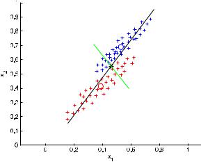
Fig. 8.8 A two-class classification problem in which we wish to reduce the data dimension to one. The standard PCA result is given as the black axis passing through the pooled data mean, and the LDA result is given by the green axis
8.8 LDA-Based 3D Face Recognition
One reason that PCA-based approaches have been popular is that they can operate with only one training example per subject. This is because it does not take account of the per-subject (within-class) distribution of the training data. However, because of this reason, the projection axes computed by PCA may make class discrimination difficult. Indeed, in the worst case for some surface feature type, it could be that the very dimensions that are discarded by PCA are those that provide good discrimination between classes. With the advent of more sophisticated datasets with several (preferably many) 3D scans per subject, more sophisticated subspaces can be used, which attempt to find the linear combination of features that best separates each subject (class). This is the aim of Linear Discriminant Analysis (LDA), while simultaneously performing dimension reduction. Thus, while PCA finds the most expressive linear combinations of surface feature map dimensions (in the simplest case, depth map pixels), LDA finds the most discriminative linear combinations.
Although 3D face recognition is an inherently multi-class classification problem in a high dimensional space, it is easier to initially look at LDA for a two-class problem in a two-dimensional space and compare it to PCA. Subsequently we will look at the issues involved with high dimensional feature vectors and we will also generalize to multi-class problems.
8.8.1 Two-Class LDA
Suppose that we have the two-class, 2D problem shown in Fig. 8.8. Intuitively we want to project the data onto a direction for which there is the largest separation of the class means, relative to the within-class scatter in that same projection direction.
344 |
A. Mian and N. Pears |
A scatter matrix is simply a scaled version of a covariance matrix, and for each set of training scans, Cc , belonging to class c {1, 2}, they are formed as:
Sc = X0Tc X0c , |
(8.26) |
where X0c is a zero-mean data matrix, as described in Sect. 8.7.1 (although it is now class-specific), and nc is the number of training scans in the set Cc . We note that these scatter matrices are often expressed as a sum of outer products:
Sc |
nc |
xc )(xi |
xc)T , |
xi |
|
Cc , |
(8.27) |
(xi |
|
||||||
|
= |
− ¯ |
− ¯ |
|
|
|
i=1
where x¯ c is the mean of the feature vectors in class Cc . Given that we have two classes, the within-class scatter matrix can be formed as:
SW = S1 + S2. |
(8.28) |
The between-class scatter is formed as the outer product of the difference between the two class means:
SB = (x¯ 1 − x¯2)(x¯ 1 − x¯ 2)T . |
(8.29) |
Fisher proposed to maximize the ratio of between class scatter to within class scatter relative to the projection direction [28], i.e. solve
J (w) = |
max |
wT SB w |
(8.30) |
|
|||
w wT SW w |
|
||
with respect to the 2 × 1 column vector w. This is known as Fisher’s criterion. A solution to this optimization can be found by differentiating Eq. (8.30) with respect to w and equating to zero. This gives:
S−1S w |
− |
J w |
= |
0. |
(8.31) |
W B |
|
|
|
We recognize this as a generalized eigenvalue-eigenvector problem, where the eigenvector of S−W1SB associated with its largest eigenvalue (J ) is our desired optimal direction, w . (In fact, the other eigenvalue will be zero because the between class scatter matrix, being a simple outer product, can only have rank 1.) Figure 8.8 shows the very different results of applying PCA to give the most expressive axis for the pooled data (both classes), and applying LDA which gives a near orthogonal axis, relative to that of PCA, for the best class separation in terms of Fisher’s criterion. Once data is projected into the new space, one can use various classifiers and distance metrics, as described earlier.
8.8.2 LDA with More than Two Classes
In order to extend the approach to a multiclass problem (K > 2 classes), we could train pairwise binary classifiers and classify a test 3D face according to the class that gets most votes. This has the advantage of finding the projection that

8 3D Face Recognition |
345 |
best separates each pair of distributions, but often results in a very large number of classifiers in 3D face recognition problems, due to the large number of classes (one per subject) often experienced. Alternatively one can train K one-versus-all classifiers where the binary classifiers are of the form subject X and not subject X. Although this results in fewer classifiers, the computed projections are usually less discriminative.
Rather than applying multiple binary classifiers to a multi-class problem, we can generalize the binary LDA case to multiple classes. This requires the assumption that the number of classes is less than or equal to the dimension of the feature space (i.e. K ≤ m where m is the dimension of our depth map space or surface feature map space). For high dimensional feature vectors, such as encountered in 3D face recognition, we also require a very large body of training data to prevent the scatter matrices from being singular. In general, the required number of 3D face scans is not available, but we address this point in the following subsection.
The multi-class LDA procedure is as follows: Firstly, we form the means of each class (i.e. each subject in the 3D face dataset). Using these means, we can compute the scatter matrix for each class using Eqs. (8.26) or (8.27). For the within-class scatter matrix, we simply sum the scatter matrices for each individual class:
K |
|
SW = Si . |
(8.32) |
i=1 |
|
This is an m × m matrix, where m is the dimension of the feature vector. We form the mean of all training faces, which is the weighted mean of the class means:
K
x¯ = 1 ni x¯ i , (8.33) n i=1
where ni is the number of training face scans in each class and n is the total number of training scans. The between-class scatter matrix is then formed as:
SB |
|
K |
x)(xi |
x)T . |
(8.34) |
= |
ni (xi |
||||
|
¯ |
− ¯ ¯ |
− ¯ |
|
i=1
This scatter matrix is also m × m. Rather than finding a single m-dimensional vector to project onto, we now seek a reduced dimension subspace in which to project our data, so that a feature vector in the new subspace is given as:
|
|
x˜ = WT x. |
|
(8.35) |
||
We formulate Fisher’s criterion as: |
|
|
|
|||
J (W) |
= |
max |
|WT SB W| |
, |
(8.36) |
|
|WT SW W| |
||||||
|
W |
|
|
|||
where the vertical lines indicate that the determinant is to be computed. Given that the determinant is equivalent to the product of the eigenvalues, it is a measure of the square of the scattering volume. The projection matrix, W, maps the original