Материал: [2.1] 3D Imaging, Analysis and Applications-Springer-Verlag London (2012)

6. Form the Weingarten matrix as:

7.Determine the principal curvatures, κ1, κ2 as the eigenvalues of the Weingarten matrix.

8.Form the Gaussian curvature, mean curvature and shape index, as required, using Eqs. (8.39) and (8.40).

Of course there are many variants of this approach. For example, in step 2, it is faster to compute normals using cross products rather than SVD, in which case we would use an arbitrary local basis to do the quadratic surface fit.

8.10 Recent Techniques in 3D Face Recognition

In this section we present a selection of promising recent techniques in the field of 3D face recognition including 3D face recognition using Annotated Face Models (AFMs) [51], local feature-based 3D face recognition [65], and expression-invariant 3D face recognition [15].

8.10.1 3D Face Recognition Using Annotated Face Models (AFM)

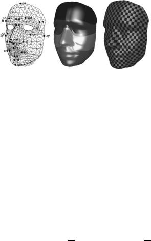
Kakadiaris et al. [50, 51] proposed a deformable Annotated Face Model (AFM), which is based on statistical data from 3D face meshes and anthropometric landmarks identified in the work of Farkas [32]. Farkas studied 132 measurements on the human face and head which are widely used in the literature. For example, DeCarlo and Metaxas [26] used 47 landmarks and their associated distance/angular measurements to describe a 3D deformable face model for tracking. Kakadiaris et al. [51] associated a subset of the facial anthropometric landmarks [32] with the vertices of the AFM and using knowledge of the facial physiology, segmented the AFM into different annotated areas. Figure 8.12 illustrates the AFM.

The input data is registered to the AFM using a multistage alignment procedure. Firstly, spin images [49] are used to coarsely align the data with the AFM. In the second step, the ICP algorithm [9] is used to refine the registration. In the final step, the alignment is further refined using Simulated Annealing to minimize the z-buffer difference. The z-buffers uniformly resample the data resulting in better registration. Uniform sampling was also used by Mian et al. [64] for better pose correction in an iterative approach. The AFM is fitted to the registered data using an elastically deformable model framework [62]. Additional constraints were imposed on the AFM similar to DeCarlo and Metaxas [26] to ensure that the fitting result is anthropometrically correct. Kakadiaris et al. [51] used a Finite Element Approximation to solve this equation and used a subdivision surface [60] as the model for greater flexibility

Fig. 8.12 Anthropometric landmarks on a 3D face mesh. Annotated Face Model (AFM) with different annotated areas shown different shaded. Demonstration of parameterization using a checkerboard texture mapped on the AFM. Figure courtesy of [50]

(compared to parametric surfaces). To speed up the fitting process, space partitioning techniques are used to reduce the cost of the nearest neighbor search per model vertex required at each iteration.

After the fitting, a continuous UV parameterization was applied to the AFM (polygonal mesh) transforming it to an equivalent geometry image. The geometry image has three channels each recording one of the three x, y or z position coordinates of the fitted AFM points. However, most of the information is contained in the z channel. Mapping between the AFM and the deformation image is performed using a spherical mapping function such that the ratio of area in 3D space to the area in UV space is approximately the same for every part of the surface.

A three channel (X, Y, Z) normal map is also extracted from the geometry image. The geometry and normal map images are treated as separate images and their individual wavelet coefficients are computed. Haar wavelets were used to extract features from the normal and geometry images. Additionally, the pyramid transform was also used to extract features from only the geometry images.

The Haar wavelet transform consisted of the tensor product of the 1D Walsh

tensor product resulted in the four channel filter bank gT g, gT h, hT g and hT h, which were applied to the images and the same subset of coefficients were used directly for comparison of two faces.

The pyramid transform [75] performs a linear multiscale, multiresolution image decomposition. The image is first divided into high and low-pass subbands and the latter is passed through a set of steerable bandpass filters resulting in a set of oriented subbands and a lower-pass subband. The latter is subsampled by a factor of two and recursively passed through the set of steerable bandpass filters resulting in a pyramid representation which is translation and rotation-invariant. These properties provide robustness to facial expressions. Kakadiaris et al. [51] applied 3 scale, 10 orientations decomposition and used the oriented subbands at the farthest scale only for comparison of two faces.

The AFM 3D face recognition system was evaluated on the FRGC v2 dataset and the Haar wavelet performed slightly better than the pyramid transform with approximately 97 % verification rate at 0.1 % FAR, as compared to 95 %. A fusion

of the two transforms provided a marginal improvement of around 0.3 % over Haar wavelets alone. If the evaluation was limited to neutral expressions, a reasonable verification scenario, verification rates improved to as high as 99 %. A rank-1 identification rate of 97 % was reported.

8.10.2 Local Feature-Based 3D Face Recognition

Three-dimensional face recognition algorithms that construct a global representation of the face using the full facial area are often termed holistic. Often, such methods are quite sensitive to pose, facial expressions and occlusions. For example, a small change in the pose can alter the depth maps and normal maps of a 3D face. This error will propagate to the feature vector extraction stage (where a feature vector represents a 3D face scan) and subsequently affect matching. For global representation and features to be consistent between multiple 3D face scans of the same identity, the scans must be accurately normalized with respect to pose. We have already discussed some limitations and problems associated with pose normalization in Sect. 8.5.5. Due to the difficulty of accurate localization of fiducial points, pose normalization is never perfect. Even the ICP based pose normalization to a reference 3D face cannot perfectly normalize the pose with high repeatability because dissimilar surfaces have multiple comparable local minima rather than a single, distinctively low global minimum. Another source of error in pose normalization is a consequence of the non-rigid nature of the face. Facial expressions can change the curvatures of a face and displace fiducial points leading to errors in pose correction.

In contrast to holistic approaches, a second category of face recognition algorithms extracts local features [96] from faces and matches them independently. Although local features have been discussed before for the purpose of fiducial point localization and pose correction, in this section we will focus on algorithms that use local features for 3D face matching. In case of pose correction, the local features are chosen such that they are generic to the 3D faces of all identities. However, for face matching, local features may be chosen such that they are unique to every identity.

In feature-based face recognition, the first step is to determine the locations from where to extract the local features. Extracting local features at every point would be computationally expensive. However, detecting a subset of points (i.e. keypoints) over the 3D face can significantly reduce the computation time of the subsequent feature extraction and matching phases. Uniform or arbitrary sparse sampling of the face will result in features that are not unique (or sufficiently descriptive) resulting in sub-optimal recognition performance. Ideally keypoints must be repeatedly detectable at locations on a 3D face where invariant and descriptive features can be extracted. Moreover, the keypoint identification (if required) and features should be robust to noise and pose variations.

8.10.2.1 Keypoint Detection and Local Feature Matching

Mian et al. [65] proposed a keypoint detection and local feature extraction algorithm for 3D face recognition. Details of the technique are as follows. The point cloud is first resampled at uniform intervals of 4 mm on the x, y plane. Taking each sample point p as a center, a sphere of radius r is used to crop a local surface from the face. The value of r is chosen as a trade-off between the feature’s descriptiveness and sensitivity to global variations, such as those due to varying facial expression. Larger r will result in more descriptive features at the cost of being more sensitive to global variations and vice-versa.

This local point cloud is then translated to zero mean and a decorrelating rotation is applied using the eigenvectors of its covariance matrix, as described earlier for full face scans in Sect. 8.7.1. Equivalently, we could use SVD on the zero-mean data matrix associated with this local point cloud to determine the eigenvectors, as described in Sect. 8.7.2. The result of these operations is that the local points are aligned along their principal axes and we determine the maximum and minimum coordinate values for the first two of these axes (i.e. the two with the largest eigenvalues). This gives a measure of the spread of the local data over these two principal directions.

We compute the difference in these two principal axes spreads and denote it by δ. If the variation in surface is symmetric as in the case of a plane or a sphere, the value of δ will be close to zero. However, in the case of asymmetric variation of the surface, δ will have a value dependent on the asymmetry. The depth variation is important for the descriptiveness of the feature and the asymmetry is essential for defining a local coordinate basis for the subsequent extraction of local features.

If the value of δ is greater than a threshold t1, p qualifies as a keypoint. If t1 is set to zero, every point will qualify as a keypoint and as t1 is increased, the total number of keypoints will decrease. Only two thresholds are required for keypoint detection namely r and t1 which were empirically chosen as r1 = 20 mm and t1 = 2 mm by Mian et al. [65]. Since the data space is known (i.e. human faces), r and t1 can be chosen easily. Mian et al. [65] demonstrated that this algorithm can detect keypoints with high repeatability on the 3D faces of the same identity. Interestingly, the keypoint locations are different for different individuals providing a coarse classification between different identities right at the keypoint detection stage. This keypoint detection technique is generic and was later extended to other 3D objects as well where the scale of the feature (i.e. r ) was automatically chosen [66].

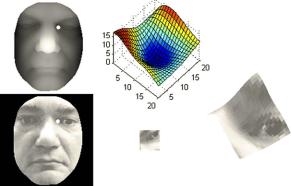
In PCA-based alignment, there is an inherent two-fold ambiguity. This is resolved by assuming that the faces are roughly upright and the patch is rotated by the smaller of the possible angles to align it with its principal axis. A smooth surface is fitted to the points that have been mapped into a local frame, using the approximation given in [27] for robustness to noise and outliers. The surface is sampled on a uniform 20 × 20 xy lattice. To avoid boundary effects, a larger region is initially cropped using r2 > r for surface fitting using a larger lattice and then only the central 20 × 20 samples covering the r region are used as a feature vector of dimension 400. Note that this feature is essentially a depth map of the local surface defined

Fig. 8.13 Illustration of a keypoint on a 3D face and its corresponding texture. Figure courtesy of [65]

in the local coordinate basis with the location of the keypoint p as origin and the principal axes as the direction vectors. Figure 8.13 shows a keypoint and its local corresponding feature.

A constant threshold t1 usually results in a different number of keypoints on each 3D face scan. Therefore, an upper limit of 200 is imposed on the total number of local features to prevent bias in the recognition results. To reduce the dimensionality of the features, they are projected to a PCA subspace defined by their most significant eigenvectors. Mian et al. [65] showed that 11 dimensions are sufficient to conserve 99 % of the variance of the features. Thus each face scan is represented by 200 features of dimension 11 each. Local features from the gallery and probe faces are projected to the same 11 dimensional subspace and whitened so that the variation along each dimension is equal. The features are then normalized to unit vectors and the angle between them is used as a matching metric.

For a probe feature, the gallery face feature that forms the minimum angle with it is considered to be its match. Only one-to-one matches are allowed i.e. if a gallery feature matches more than one probe feature, only the one with the minimum angle is considered. Thus gallery faces generally have a different number of matches with a probe face.

The matched keypoints of the probe face are meshed using Delaunay triangulation and its edges are used to construct a similar 3D mesh from the corresponding keypoints of the gallery face. If the matches are spatially consistent, the two meshes will be similar (see Fig. 8.14). The similarity between the two meshes is given by:

i

where εpi and εgi are the lengths of the corresponding edges of the probe and gallery meshes, respectively. The value nε is the number of edges. Note that γ is invariant to pose.

A fourth similarity measure between the faces is calculated as the mean Euclidean distance d between the corresponding vertices (keypoints) of the meshes after least squared minimization. The four similarity measures namely the average