Материал: [2.1] 3D Imaging, Analysis and Applications-Springer-Verlag London (2012)

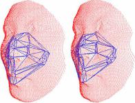
Fig. 8.14 Graph of feature points matched between two faces. Figure courtesy of [65]

angle between the matching features, the number of matches, γ and d are normalized on a scale of 0 to 1 and combined using a confidence weighted sum rule:

where κx is the confidence in individual similarity metric defined as a ratio between the best and second best matches of the probe face with the gallery. The gallery face with the minimum value of s is declared as the identity of the probe. The algorithm achieved 96.1 % rank-1 identification rate and 98.6 % verification rate at 0.1 % FAR on the complete FRGC v2 data set. Restricting the evaluation to neutral expression face scans resulted in a verification rate of 99.4 %.

8.10.2.2 Other Local Feature-Based Methods

Another example of local feature based 3D face recognition is that of Chua et al. [21] who extracted point signatures [20] of the rigid parts of the face for expression robust 3D face recognition. A point signature is a one dimensional invariant signature describing the local surface around a point. The signature is extracted by centering a sphere of fixed radius at that point. The intersection of the sphere with the objects surface gives a 3D curve whose orientation can be normalized using its normal and a reference direction. The 3D curve is projected perpendicularly to a plane, fitted to the curve, forming a 2D curve. This projection gives a signed distance profile called the point signature. The starting point of the signature is defined by a vector from the point to where the 3D curve gives the largest positive profile distance. Chua et al. [21] do not provide a detailed experimental analysis of the point signatures for 3D face recognition.

Local features have also been combined with global features to achieve better performance. Xu et al. [90] combined local shape variations with global geometric features to perform 3D face recognition. Finally, Al-Osaimi et al. [4] also combined local and global geometric cues for 3D face recognition. The local features represented local similarities between faces while the global features provided geometric consistency of the spatial organization of the local features.

8.10.3 Expression Modeling for Invariant 3D Face Recognition

Bronstein et al. [15] developed expression-invariant face recognition by modeling facial expressions as surface isometries (i.e. bending but no stretching) and constructing expression-invariant representations of faces using canonical forms. The facial surface is treated as a deformable object in the context of Riemannian geometry. Assuming that the intrinsic geometry of the facial surface is expressioninvariant, an isometry-invariant representation of the facial surface will exhibit the same property.

The Gaussian curvature of a surface is its intrinsic property and remains constant for isometric surfaces. (Clearly, the same is not true for mean curvature.) By isometrically embedding the surface into a low-dimensional space, a computationally efficient invariant representation of the face is constructed. Isometric embedding consists of measuring the geodesic distances between various points on the facial surface followed by Multi-Dimensional Scaling (MDS) to perform the embedding.

Once an invariant representation is obtained, comparing deformable objects, such as faces, becomes a problem of simple rigid surface matching. This, however, comes at the cost of loosing some accuracy because the facial surface is not perfectly isometric. Moreover, isometric modeling is only an approximation and can only model facial expressions that do not change the topology of the face, such as an open mouth.

Given a surface in discrete form, consisting of a finite number of sample points on surface S, the geodesic distances between the points dij = d(xi , xj ) are measured and described by the matrix D. The geodesic distances are measured with O(N ) complexity using a variant of the Fast Marching Method (FMM) [80] which was extended to triangular manifolds in [52]. The FMM variant used was proposed by Spira and Kimmel [83] and has the advantage that it performs computation on a uniform Cartesian grid in the parameterization plane rather than the manifold itself.

Bronstein et al. [15] numerically measured the invariance of the isometric model by placing 133 markers on a face and tracking the change in their geodesic and Euclidean distances due to facial expressions. They concluded that the change in Euclidean distances was two times greater than the change in geodesic distances. Note that the change in geodesic distances was not zero.

The matrix of geodesic distances D itself can not be used as an invariant representation because of the variable sampling rates and the order of points. Thus the Riemannian surface is represented as a subset of some manifold Mm which preserves the intrinsic geometry and removes the extrinsic geometry. This is referred to as isometric embedding. The embedding space is chosen to simplify the process. Bronstein et al. [15] treat isometric embedding as a simple mapping:

between two surfaces such that the geodesic distances between any two points in the original space and the embedded space are equal. In the embedding space, geodesic distances are replaced by Euclidean distances. However, in practice, such an embed-

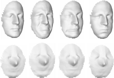
Fig. 8.15 The canonical representations (second row) are identical even though the original face surface is quite different due to facial expressions (top row). (Image courtesy of [15])

ding does not exist. Therefore, Bronstein et al. [15] try to find an embedding that is near-isometric by minimizing the embedding error given by:

where dij and dij are the distances between points i, j in the embedding and original spaces respectively. X = (x1, x2, . . . , xN ) is an N by m matrix of parametric coordinates in Mm and W = (wij ) is a symmetric matrix of weights determining the relative contribution of the distances between all pairs of points to the total error. The minimization of the above error with respect to X can be performed using gradient descent.

In addition to the limitations arising from the assumptions discussed above, another downside of this approach is that the isometric embedding also attenuates some important discriminating features which are not caused by expressions. For example, the 3D shape of the nose and the eye sockets is somewhat flattened. Figure 8.15 shows sample 3D faces of the same person. Although the facial surface changes significantly in the original space due to different facial expressions, the corresponding canonical representations in the embedded space look similar.

The approach was evaluated on a dataset consisting of 30 subjects with 220 face scans containing varying degrees of facial expression. The gallery consisted of neutral expressions only and the results were compared with rigid face matching [15].

8.10.3.1 Other Expression Modeling Approaches

Another example of facial expression modeling is the work of Al-Osaimi et al. [5]. In this approach, the facial expression deformation patterns are first learned using a linear PCA subspace called an Expression Deformation Model. The model is learnt using part of the FRGC v2 data augmented by over 3000 facial scans under different facial expressions. More specifically, the PCA subspace is built from shape residues between pairs of scans of the same face, one under neutral expression and the other under non-neutral facial expression. Before calculating the residue, the two scans are first registered using the ICP [9] algorithm applied to the semi-rigid regions of the faces (i.e. forehead and nose). Since the PCA space is computed from the residues, it only models the facial expressions as opposed to the human face.

The linear model is used during recognition to morph out the expression deformations from unseen faces leaving only interpersonal disparities. The shape residues between the probe and every gallery scan are calculated. Only the residue of the correct identity will account for the expression deformations and other residues will also contain shape differences. A shape residue r is projected to the PCA subspace E as follows:

If the gallery face from which the residue was calculated is the same as the probe, then the error between the original and reconstructed shape residues

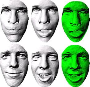
will be small, otherwise it will be large. The probe is assigned the identity of the gallery face corresponding to the minimum value of ε. In practice, the projection is modified to avoid border effects and outliers in the data. Moreover, the projection is restricted to the dimensions of the subspace E where realistic expression residues can exist. Large differences between r and r are truncated to a fixed value to avoid the effects of hair and other outliers. Note that it is not necessary that one of the facial expressions (while computing the residue) is neutral. One non-neutral facial expression can be morphed to another using the same PCA model. Figure 8.16 shows two example faces morphed from one non-neutral expression to another. Using the FRGC v2 dataset, verification rates at 0.001 FAR were 98.35 % and 97.73 % for face scans under neutral and non-neutral expressions respectively.

8.11 Research Challenges

After a decade of extensive research in the area of 3D face recognition, new representations and techniques that can be applied to this problem are continually being released in the literature. A number of challenges still remain to be surmounted. These challenges have been discussed in the survey of Bowyer et al. [14] and include

Fig. 8.16 Left: query facial expression. Centre: target facial expression. Right: the result of morphing the left 3D image in order to match the facial expression of the central 3D image. Figure courtesy of [5]

improved 3D sensing technology as a foremost requirement. Speed, accuracy, flexibility in the ambient scan acquisition conditions and imperceptibility of the acquisition process are all important for practical applications. Facial expressions remain a challenge as existing techniques lose important features in the process of removing facial expressions or extracting expression-invariant features. Although relatively small pose variations can be handled by current 3D face recognition systems, large pose variations often can not, due to significant self-occlusion. In systems that employ pose normalization, this will affect the accuracy of pose correction and, for any recognition system, it will result in large areas of missing data. (For profile views, this may be mitigated by the fact that the symmetrical face contains redundant information for discrimination.) Additional problems with capturing 3D data from a single viewpoint include noise at the edges of the scan and the inability to reliably define local regions (e.g. for local surface feature extraction), because these become eroded if they are positioned near the edges of the scan. Dark and specular regions of the face offer further challenges to the acquisition and subsequent preprocessing steps.

In addition to sensor technology improving, we expect to see improved 3D face datasets, with larger numbers of subjects and larger number of captures per subject, covering a very wide range of pose variation, expression variation and occlusions caused by hair, hands and common accessories (e.g. spectacles, hats, scarves and phone). We expect to see publicly available datasets that start to combine pose variation, expression variation, and occlusion thus providing an even greater challenge to 3D face recognition algorithms.

Passive techniques are advancing rapidly, for example, some approaches may no longer explicitly reconstruct the facial surface but directly extract features from multiview stereo images. One problem with current resolution passive stereo is that there