Материал: [2.1] 3D Imaging, Analysis and Applications-Springer-Verlag London (2012)

9.4.5 DTM from Statistical Properties of the Point Cloud

Unsupervized statistical filtering algorithms are an alternative to object-based filtering. Separation of ground and object points within the LIDAR point cloud is a prerequisite for DTM generation. Bartels and Wei [17] developed a LIDAR filtering technique, purely based on the statistical distribution of the point cloud. For the definition of the algorithm, three assumptions can be made to exploit the statistics of a 2.5 dimensional point cloud.

•From a global perspective, there is a normal distribution of ground point elevation, similar to samples collected from a population [40].

•Object points may disturb or ‘skew’ this normal distribution [16].

•The number of visible ground points must dominate the LIDAR point cloud to ensure validity of the first assumption.

The last assumption is essential to avoid misclassification of object points as ground points, for example, large flat roofs in dense urban areas. Furthermore, there has to be a minimum number of LIDAR ground points available to be able to make a solid statistical statement over the point cloud’s distribution. Based on these assumptions, the unsupervized object and ground point separator is formulated [17]. First, the skewness of the point cloud is calculated. If it is greater than zero, peaks (i.e. objects) dominate the point cloud distribution. The greatest value of the point cloud is then removed by classifying it as an object point. These steps are iteratively executed while the skewness of the point cloud is greater than zero. Finally, the remaining points are normally distributed and belong to the ground. By doing so, the skewed distribution of the data is balanced, and the algorithm is therefore called Skewness Balancing [16].

A limitation of the basic algorithm is the assumption that object points are located above the ground. This is valid for large classes of terrain types, but in mountainous areas, the algorithm would misclassify ground points as object points. Skewness balancing is therefore extended to sloped terrain with the following reasoning. After termination of basic skewness balancing on the original positively skewed LIDAR point cloud, the extracted subset of LIDAR points (which still contains misclassified ground points) can still be positively skewed. The remaining object point cloud is now re-considered as a new model, DSM*, which is statistically independent from the original DSM. It is now re-filtered by skewness balancing and misclassified ground points are thus iteratively corrected. The extended algorithm terminates as the remaining object points converge to zero, as depicted in Fig. 9.13.

The advantages of this unsupervized approach are obvious: skewness balancing does not require pre-defined thresholds, a pre-determined number of iterations or tunable (i.e. application-dependent) weighting factors. It does not incorporate prior knowledge about the terrain or objects and is independent from format (gridded or non-gridded) and resolution of the data. Ground points between gaps and in narrow streets are picked up without thinning out the data. In doing so, object and terrain details are preserved. Skewness balancing is therefore ideal for integration

Fig. 9.13 Skewness balancing algorithm and adaptation to sloped terrain [17]. Left: Original algorithm. Right: Adapted to sloped terrain

into GIS software packages, while having the option to improve it by deriving an optimization-localization operator.

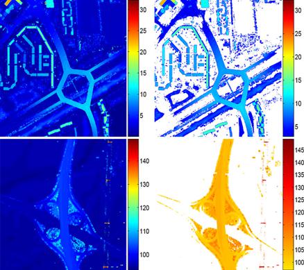
Figure 9.14 depicts a large number of key terrain elements in rural and urban area filtered out by the algorithm. Bare earth (streets, pavements and court yards), detached objects (buildings and vegetation) and ambiguously attached objects (bridges, motorway junctions, ramps and slopes) are separated from the two tiles of LIDAR point clouds. Figure 9.14(bottom left) shows that skewness balancing even picks up power transmission lines, while vegetation in rural and forestry areas is correctly filtered at an accuracy of 96 % [19].

To create a DEM or DTM after the object points are removed from LIDAR point cloud, the following possibilities should be taken into account, and a proper approach should be taken accordingly.

•For areas where high vegetation are removed, the corresponding LIDAR LE can be used for filling the patches because the LIDAR can penetrate vegetation.

•For areas where the removed points represent buildings or other hard objects, there are two situations.

–For those areas with reasonable size, TIN linear interpolation, bilinear interpolation, and Kriging interpolation [181] could be used to fill the empty space.

–For a large area where object points are removed, the true information of terrain is unknown. The common practice is to leave the space as empty (data missing).

Fig. 9.14 DSM (left column) and filtered object points (right column) obtained from skewness balancing of two different LIDAR tiles. Top: Thamesmead, London, UK (courtesy of Environment Agency, UK). Bottom: Mannheim, Germany (courtesy of TopoSys GmbH and the Stadt Mannheim, Germany)

9.5 Research Challenges

With the development of remote sensing technology and advanced signal processing algorithms, 3D DEM generation from remote sensing has demonstrated enormous potential with advantages of automation, economy, and large coverage of terrain. Related techniques have been maturing due to significant investment in sensing devices, instruments, processing algorithms, and software development. The launch of Earth observation satellites, such as, Envisat, Landsat, GeoEye, and Worldview has brought opportunities as well as challenges to the research communities.

•When the high accuracy, high resolution, and high density data are continuously acquired from various Earth observation satellites, huge datasets are generated. How to store and retrieve these datasets is the first challenge. These may require reliable servers and tangible databases for data storage, and robust algorithms for information retrieval from the databases if needed.

•For DEM generation from stereoscopic imagery, further improving DEM accuracy requires better mathematical models which can adaptively correct errors caused by sensors’ platform attitude instability and geometric distortion of images. Automation demands more robust algorithms for image matching processes.

•As described previously, most current techniques used in 3D DEM generation from remote sensing need intensive interaction from operators. They are timeconsuming and the accuracy of the final product is difficult to control. This demands researchers’ further understanding of physical properties of sensing elements (e.g. SAR) with accurate theoretical models for signal interpretation, and better knowledge of satellite orbits and imaging geometry (for both stereo images and SAR images).

•For LIDAR, power consumption is the key issue for spaceborne missions although lasers can provide more accurate elevation data compared with other devices. Quantitative analysis of the effects caused by weather and atmospheric conditions to LIDAR is required to ensure that the raw signal/data is interpreted correctly.

The above aspects need to be addressed in order to bring more automation and higher accuracy to the DEMs generated from remote sensing.

9.6 Concluding Remarks

In this chapter, three methods used for 3D DEM generation from remote sensing have been introduced. These are DEM generation from optical stereoscopic imagery, InSAR, and airborne LIDAR. All of these have shown enormous potential in many application areas. After working through this chapter, it is expected that readers appreciate the achievements and are aware of the problems remaining in this research area. Readers should have sufficient knowledge to answer the questions presented in Sect. 9.8 and carry out the exercises in Sect. 9.9, with the comprehensive references listed at the end of this chapter. Also, readers should be able to do the following.

•Outline processing procedures of DEM generation from satellite stereoscopic imagery, InSAR, and airborne LIDAR.

•Explain how the 3D passive vision technology developed in the computer vision community (Chap. 2) can be applied to DEM generation from satellite stereoscopic imagery.

•Explain how the 3D active vision technology can be used for DEM generation from InSAR and LIDAR.

•Appreciate various algorithms developed in the area of DEM generation for stereo-matching, image registration, phase unwrapping, and data filtering.

•Estimate DEM accuracy based on knowledge of imaging geometry and relative physical properties of sensing devices.