Материал: [2.1] 3D Imaging, Analysis and Applications-Springer-Verlag London (2012)

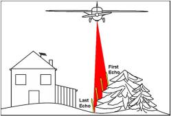
Fig. 9.11 LIDAR acquisition principle

landslide prediction, corridor mapping and wave propagation models for mobile telecommunication networks.

From an airborne platform, a LIDAR system estimates the distance between the instrument and a point on the surface by measuring the time for a round-trip of a laser pulse, as illustrated in Fig. 9.11. Differential Global Positioning System (DGPS) and Inertial Navigation System (INS) complement the data with position and orientation, respectively [78]. The result is the collection of surface height information in the form of a dense 3D point cloud. LIDAR is an active sensor which relies on the amount of backscattered light. The portion of light returning back to the receiver depends on the scene surface type illuminated by the laser pulse. Consequently, there will be gaps and overlaps in the data which is therefore not homogeneously and regularly distributed [14]. Additionally, since LIDAR is an active sensor and is independent of external lighting conditions, it can be used at night, a great advantage compared to traditional stereo matching [93]. Typical flight heights range from 600 m to 950 m [14, 81], scan angles 7–23◦, wavelengths 1047–1560 nm, scan rates 13–653 Hz, and pulse rates 5–83 kHz [25, 78]. Average footprint sizes range typically from 0.4–1.0 m, depending on the flight height [20, 91]. Scan and pulse rates, in particular, have grown in recent years, leading to higher point densities as a function of flight height, velocity of the aircraft, scan angle, pulse rate and scan rate [10, 13].

The capability of the laser to penetrate gaps in vegetation allows the measurement of occluded ground. This is due to the laser’s large footprint relative to the vegetation gaps. At least the First Echo (FE) and the Last Echo (LE) can be recorded, as schematically depicted in Fig. 9.11. Ideally, the FE and LE are arranged in two different point clouds as subsets within LIDAR data [122] and clearly the differentiation of multiple echoes is a challenge. Modern LIDAR systems can record up to four echoes (or more if derived from full waveform datasets), while the latest survey techniques, such as low-level LIDAR, allow point densities up to 100 points per square meter [28]. The latest developments of the full waveform LIDAR have introduced a new range of applications. The recording of multiple echoes allows modeling of the vertical tree profile [14]. Acquired FE points mostly comprise canopies, sheds, roofs, dormers and even small details such as aerials or chimneys, whereas LEs are reflections of the ground or other lower surfaces after the laser has

penetrated gaps within the foliage. The occurrence of multiple echoes at the same geo-referenced point indicates vegetation but also edges of hard objects [10]. The difference between FE and LE therefore reveals, in the best case, building outlines and vegetation heights [138]. Table 9.3 summarizes the pros and cons of LIDAR versus traditional aerial photogrammetric techniques.

9.4.2 Accuracy, Error Types and Countermeasures

LIDAR is the most accurate remote sensing source for capturing height. It has revolutionized photogrammetry with regard to vertical accuracy, with values ranging between 0.10–0.26 m [3, 4, 34, 74, 104, 107, 167, 179]. Like any other physical measurements, LIDAR errors are composed of both systematic and random errors. Systematic errors are due to the setting of the equipment; generally they have a certain pattern and are therefore reproducible. Examples are systematic height shifts as a function of flight height, which are due to uncertainty of GPS, georeferencing and orientation. Time errors of assigning range and position are reported to be <10 μs [167]. Calibration can be carried out by using known mounting angles, the redundancy from overlapping (crossing) strips and ground truth (i.e. manually measured

GCPs which have been acquired in an accompanying field survey). Problems occur if the positions of GCPs and measured LIDAR points do not correspond with each other [137]. This can be solved using a high point density, acquired with a low altitude, low velocity and a steep scan angle.

In contrast, random errors are not reproducible and are thus more difficult to eliminate. Gross errors, blunders and ‘no data’ situations are due to a temporal malfunction of the LRF or occasional perturbations such as birds or low flying aircrafts [143]. Data voids are due to the irregular sampling nature of the LIDAR and have to be corrected using interpolation if required. The total number of gross errors and blunders may be small, but their overall impact on the data is strong. Kidner et al. [89] reported that local blunders can be large as 20 m and can be detected if the height of all neighbouring points is below a certain threshold, for example ≤5 m. Extreme blunders can be greater than 767 m [89] and can be removed by comparing the mean and standard deviation of the height differences of each LIDAR point in a defined neighborhood.

Point density and scan range per scanned line are a function of scan angle, however it is also known that the greater the scan angle the greater its elevation error [179]. The error caused by the scan angle becomes smaller when the flight height and pulse rate are lower [7]. A small scan angle ensures that terrain or object edges are resolved more clearly and vertical tree profiles can be sampled due to the fact that laser pulses reach lower tree branches [104]. In general, the smaller the scan angle, the higher the point density, the better the edges on man-made structure are sampled, and the better the laser can be pushed forward to lower branch levels of trees [138].

Multipath propagation causes backscattered laser light to travel a longer time. Consequently, some points will appear below the actual surface [91, 143]. Multipath effects of LE LIDAR data can be compensated for by exploiting the redundant information of FE and LE [166].

Finally, wind, atmospheric distortions and bright sunlight can all influence the accuracy of LIDAR data as the laser beam is narrow [12]. The best laser ranging conditions are achieved if the weather is dry, cool and clear [12]. Furthermore, water vapour and humidity such as rain and fog attenuate the power of the laser. This disturbing effect can be deliberately exploited for investigating clouds and aerosols in the atmosphere using ground-based LIDAR [77]. To generalize, studies have revealed that the greater slope, terrain roughness, amount of vegetation and the larger the flight velocity and height, the smaller the scan angle, the larger the random error will be [14, 74, 93, 179].

To reduce inaccuracies within the acquired data, error models are applied. A popular method to estimate the total error can be done by calculating the Root Mean Square Error (RMSE) of equal georeferenced GCPs and LIDAR points as defined in [74]:

where NGCP is the total number of GCPj and Xj the corresponding LIDAR points with j {1, 2, . . . , NGCP}. To break the absolute error down, mean height differences (systematic error) and standard deviation of difference (random error) can be calculated. Yu [179] observed that the random error decreases at greater vegetation penetration rates (i.e. the more open the space is), greater point densities and lower flight heights, while the systematic error remains stable at different flight heights. Even if there is no initial vertical error evident, a horizontal error still has an impact on the vertical error. Hodgson et al. [75] established a link between the terrain slope angle α and the horizontal displacement eh of the LIDAR point yielding the vertical error ev :

where the horizontal error eh is dominated by the flight height h, which is a general rule of thumb [74]

Systematic and random errors can be corrected by GCPs, surveyed at the same time with LIDAR data. From another point of view, LIDAR itself can be used to provide GCPs for accuracy assessment of photogrammetric products as recently demonstrated by James et al. [84]. Systematic errors can either be eliminated by careful calibration or, if known, calculated and removed from the error budget. Random errors can only be estimated after the survey in a post-processing analysis. Table 9.4 summarizes all typical systematic and random errors and states countermeasures.

9.4.3 LIDAR Interpolation

In general, there are two principal ways to prepare LIDAR data for filtering techniques: gridding or working on the original point cloud. On the one hand, some researchers suggest the use of the original data for accuracy reasons, since gridding and interpolation may omit original data and induce additional non-existent data. On the other hand, gridding and interpolation allows the use and further advancement of well-known image processing techniques [47], such as filtering in the spatial and frequency domain. For applications requiring data fusion, different bands have to be co-registered to obtain a consistent format. Typical spatial resolutions for gridding are in the order of 0.25–2 m [104]. Commonly used interpolation techniques include nearest neighborhood and bilinear interpolation [34, 111, 146, 167, 181].

Bater et al. [20] compared seven interpolation methods applied to LIDAR data at different resolutions and measured the interpolation error as RMSE. Conclusions were that, although the interpolation error is independent of the interpolation method, it is a function of the resolution, where 0.5 m increase in spatial resolution yields an RMSE increase of 1 cm on average. Therefore, the authors suggested employing a natural neighbor algorithm with minimal interpolation error and computational costs. Natural or nearest neighbor interpolation suggests that missing data can be synthesized by the mean (or median) of adjacent data points based on the assumption that they are similar.

9.4.4 LIDAR Filtering

The main interest in airborne LIDAR data is to generate accurate elevation maps and to identify objects within the point cloud. The main products include Digital Surface Models (DSM), Digital Terrain Models (DTM) and normalized DSMs (nDSM) [143]. A DSM includes all sampled top surfaces of objects and ground [14, 136, 138], including tree canopies, roof tops, chimneys or above ground power transmission lines, as illustrated in Fig. 9.12. A DSM can also be directly produced from the LIDAR point cloud. Since many applications require accurate ground data, one major goal in LIDAR filtering is to separate object and ground points. If object points are of interest, an nDSM can then be generated very conveniently by subtracting the DTM from the DSM [172]. Again, an interpolation step is required to create a DEM from the filtered data (to fill those patches where objects were with appropriate data).

LIDAR filtering is the bottle-neck in the processing chain from acquisition to real applications. Friess [50] reported that the ratio of post-processing to acquisition time for correcting the points’ geometry is up to 14:1 and DEM generation demands an even higher ratio of 20:1. Filtering algorithms constitute the major contribution to a final product derived from LIDAR [167], taking three times longer than the acquisition. Flood [43] reported that at least 60 % of the production time to obtain DEMs is allocated for filtering and other post-processing steps. Although LIDAR