Материал: [2.1] 3D Imaging, Analysis and Applications-Springer-Verlag London (2012)

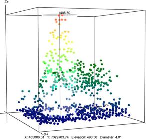
Fig. 10.5 Lidar-based individual tree height measurement, upper Tanana valley of interior Alaska, USA. Units are meters

10.3.2.1 Automated Individual Tree Measurement Using Lidar

Because LIDAR represents direct, and automatically georeferenced, digital measurements of 3D forest canopy structure, it is considerably easier to automate the individual tree detection and measurement process with LIDAR than is the case with digital photogrammetry. In fact, over the last ten years, a considerable amount of attention has been devoted to analysis of airborne LIDAR at the individual tree level. In general, these approaches tend to operate upon the high-density LIDAR canopy height model that is formed from gridding the LIDAR returns from the top of the canopy surface and subtracting the elevation of the underlying LIDAR terrain model. A variety of computer vision algorithms have been proposed for isolating the features within this canopy height model that correspond to individual tree crowns, including spectral analysis using wavelets [12], morphological watershed segmentation [20, 49], valley-following [41], and level-set analysis [21]. Of these techniques, morphological watershed segmentation is probably the most robust and widely used. This algorithm is based on the immersion process, as described in [53]. In this process, the canopy height model is inverted, and then starting at the local minima, water is poured in that fills up various catchment basins (watersheds). At each point where water from two different catchment basins merge, a dam is built. The result of the process is a complete tessellation of the image defined by the locations of the dams surrounding every watershed [53]. In a forestry context, these individual watersheds often correspond to individual tree crowns.

The morphological watershed segmentation technique can be very effective in situations where the tree crowns are distinct morphological features, even if the trees are closely spaced in a closed canopy. However, the technique is not as effective in stands where crowns are intermixed (e.g. deciduous stands). Figure 10.6

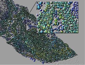
Fig. 10.6 Lidar-based individual tree crown segmentation, upper Tanana valley of interior Alaska, USA. Black circles indicate position and size of crown segments. Surface is color-coded by canopy height (blue: low canopy height, red: high canopy height). Inset shows area surround around a field plot, and green circles indicated field-measured trees

shows the result of a watershed-based individual tree crown segmentation algorithm applied to high-density airborne LIDAR collected over a boreal forest area in interior Alaska. As is evident from the inset in this graphic, which shows a comparison of the field-measured tree crowns to the watershed-based tree crowns (estimated locations and crown widths indicated by the black circles) within a 1/30th ha plot area, the segmentation algorithm successfully identified several of the larger crowns within the plot, but does not successfully delineate the smaller tree crowns that are not resolved in the 1-meter resolution LIDAR canopy height model. This algorithm also tends to over-segment in complex stands, since there is often morphological complexity even within a single tree crown

Once the forest area is segmented into individual tree crowns, the raw LIDAR can be extracted for each segment and used to obtain more detailed information on the tree. For example, the highest LIDAR return within the segment provides an estimate of the tree top [1]. In leaf-off conditions, the intensity values of the raw LIDAR returns within a crown segment can be used to classify the segment into conifer or deciduous species class. For example, Kim et al. [22] used a linear discriminant function to classify various species of trees in the Pacific Northwest of the United States using mean intensity of LIDAR returns in the upper portion of the crown as the primary metric and reported a classification rate of 83.4 % for separating coniferous and deciduous trees using leaf-off LIDAR data, and 73.1 % using leaf-on LIDAR data.

10.3.2.2Comparison of Lidar-Based and Photo-Based Individual Tree Measurements

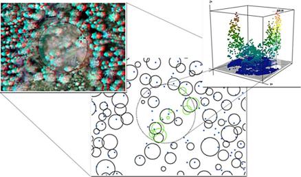
Individual tree measurements, acquired using high-density LIDAR and large-scale aerial photography, were compared to field-based measurements acquired on an inventory plot established in the upper Tanana valley of interior Alaska (Fig. 10.7). The aerial photography was acquired using a low-cost, non-metric digital single

Fig. 10.7 Comparison of photogrammetric and LIDAR individual tree height measurement techniques, upper Tanana valley of interior Alaska, USA. Center graphic shows 1/30th ha circular plot (dashed line), black circles indicate locations and estimated crown sizes from automated segmentation of LIDAR canopy height model, green circles indicate location of field-measured trees within plot, and blue dots indicate locations of individual tree crowns observed in aerial photo stereo model. Upper left inset graphic shows the plot area in stereo (red-blue glasses are needed for stereo viewing) and the black cross is positioned to measure the top of a selected tree in the plot. The upper right inset graphic shows this same tree top measured in the LIDAR point cloud (color coded by height). The field-measured height of this white spruce tree is 22.25 meters, the LIDAR-measured height is 22.03 m, and the photogrammetrically-measured height is 23.8 m. The error in the LIDAR measurement is likely due to the LIDAR pulses missing the top of the tree crown [1], while the error in the photogrammetric measurement is likely a combination of the errors in the coarse terrain model and difficulty in identifying the true elevation of the tree top when viewed in stereo

lens reflex (SLR) camera mounted on a Cessna 185 aircraft flying at approximately 1000 meters above ground level (AGL). It should also be noted that this low-cost system did not have image motion compensation. In order to remove one source of error in the comparisons, the ground control points for the exterior orientation of the non-metric imagery were acquired from the airborne LIDAR, using the FUSION interactive LIDAR measurement environment [11, 30]. The photo-based tree height measurements were acquired by the following process: (1) photogrammetrically measuring the elevations of several points on bare ground distributed throughout the area, (2) using these points to generate a terrain model, (3) photogrammetrically measuring tree top elevation for all visible trees in the area, and (4) estimating tree heights as the difference between the tree top elevation and the elevation of the underlying terrain model. Lidar-based tree height measurements were generated similarly by subtracting the elevation of the LIDAR-based terrain elevation from the elevation of the highest LIDAR return within an individual tree crown segment.

high-resolution (large-scale) digital aerial imagery can provide highly detailed information on forest type and density and at a significantly lower cost than LIDAR, but provides less accurate measurements of individual tree dimensions. It is expected that these highly complementary remote sensing systems will both play an important role in reducing the cost and increasing the efficiency of forest inventory systems in the future.

10.3.3 Area-Based Approach to Estimating Biomass with Lidar

Given the structural and compositional complexity of many forests, there is a need for alternative techniques for quantifying biomass and aboveground carbon using LIDAR that are not dependent upon accurate detection and measurement of individual tree crowns. Aggregate measures of forest structure, including basal area (m2/ha), biomass (MG/ha), and volume (m3/ha), calculated from all trees within a given area (above a certain minimum diameter) are typically highly correlated to structural metrics calculated using the LIDAR point cloud data extracted over the same area. Most of the variability in biomass within a given area can be explained by three LIDAR-derived structural metrics: (1) mean height of canopy-level LIDAR returns, (2) LIDAR-derived percent canopy cover, and (3) standard deviation of canopy-level LIDAR returns [26]. Collectively, these three metrics provide a quantitative description of the three-dimensional spatial distribution of canopy material within a given area, which in turn, is strongly related to the amount of aboveground biomass present in this area. However, many other LIDAR-derived structural metrics can be generated from the LIDAR point cloud (maximum height of canopy level returns, 10th, 25th, 50th, 75th, 90th, percentile height of canopy-level returns, canopy density by layer, etc.). For example, Fig. 10.8 shows the vertical distribution of LIDAR data, extracted LIDAR structural metrics, and the biomass level for four selected field plots in interior Alaska. Magnussen and Boudewyn established the theoretical basis for the relationship between LIDAR height quantiles and the vertical distribution of canopy materials [29]. Given the tremendous variability in forest composition and structure in forests throughout the world, the specific models describing the relationship between biomass and LIDAR metrics can also vary by forest type, and often will incorporate different predictor variables and regression coefficients. A practical approach to estimate biomass and other inventory parameters (density, volume, etc.) using LIDAR was developed in Norway [35, 36], in which field inventory data was collected at a limited number of accurately-georeferenced plots, then empirical relationships were established between field-based inventory estimates and a selection of LIDAR structural metrics extracted for the area associated with each plot. An automated variable selection procedure (stepwise regression) was used to select the predictor variables for each regression model. Figure 10.9 shows the relationship between fieldand LIDARbased estimates of (square root-transformed) aboveground tree biomass on seventynine (79) field plots established in the upper Tanana valley of interior Alaska, where the model is obtained via a stepwise regression procedure.