Материал: [2.1] 3D Imaging, Analysis and Applications-Springer-Verlag London (2012)

where (x(s, θ ), y(s, θ )) denotes a point along the ray making an angle θ with an arbitrary but fixed axis, and s is distance along the ray. We can convert this to a direct integral along the line by taking log intensities, in which case the process corresponds mathematically to a Radon transform. We are integrating the function μ(x, y) along a given line. If we have a parallel beam geometry, many such lines are integrated through the object at the same angle, θ , but different offsets, d , providing a linear projection profile, P , of the object. The 1D projection at this angle becomes:

This corresponds to the Radon transform, but to reconstruct μ(x, y) we must solve for the inverse Radon transform. There is a nice theorem that helps in this process, known as the central slice theorem or the projection slice theorem. It turns out that the 1D Fourier transform of the projection P is actually the same as a line through the 2D Fourier transform of μ(x, y). Hence, we can take the 1D Fourier transform of all our projections at different angles and use these to interpolate the full 2D Fourier transform. The final image is then obtained by a 2D inverse Fourier transform of the result.

A simpler approach is merely to back-project (spread the value associated to a line uniformly among all pixels on the line) the profiles at all angles and average them. This produces images which are rather blurred and this blurring has an analytical expression. Correct results are achieved if the individual slice spectra are filtered before undergoing a 1D inverse Fourier transform and then being projected back into the 2D spatial image. Each filtered projection is simply projected back into the 2D image at the same angle as it was taken and the sum of all projections is then averaged. This process is known as filtered back-projection. An excellent online demo is available [45].

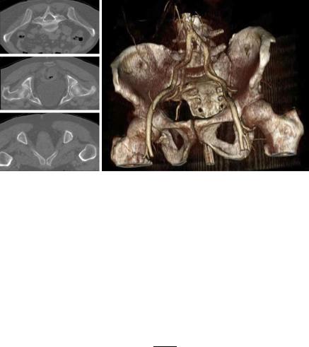
We have described how a 2D slice is produced. By incrementing the slice position, we end up with a stack of slices corresponding to the full 3D volume. In modern scanners, the reconstruction is not from parallel beams, but fan beams (single source to multiple detectors in a ring). The acquisition is often taken using a spiral motion with the patient continually moving through the scanner and reconstruction being fully 3D. An example CT scan is shown in Fig. 11.1. Multiple slices are often detected in one acquisition and the latest scanners may be 256 or even 512 slice devices. This enables, for example, coronary scans to be taken in a single heartbeat.

11.2.1.1 Characteristics of 3D CT Data

Since CT images the X-ray attenuation coefficient, it is good at imaging dense objects such as bones. The contrast for soft tissues may not be so high, but certainly fat and muscle can be differentiated and often pathological tissue such as cancerous lesions can be identified. The intensity corresponding to a given tissue density should always be the same and CT voxels are generally provided in Hounsfield units

Fig. 11.1 Slices from an abdominal CT and volume rendering showing pelvic bone and major vessels

(HU) (−1000 for air, 0 for water) or CT number (HU + 1000). Hounsfield units are named after Sir Godfrey Hounsfield, who received the Nobel Prize for Medicine in 1979 for his pioneering work in constructing the first CT scanner.

The resolution of a CT slice is generally less than 1 mm. Image dimensions are typically a power of 2 and in-slice matrix will typically be 512 × 512. The thickness and separation of slices varies depending on the application, but will typically be a few millimeters unless there is a specific desire for an accurate 3D model. Since CT consists of multiple X-rays, radiation dose is a major issue. As with X-rays, there is a compromise between image quality and dose. The relationship between dose, D, and signal-to-noise ratio (SNR) can be expressed as:

D SNR2 d3h

where d is in-plane pixel size, and h is slice thickness [16]. At the same time there is a pay-off between resolution and SNR. Greater resolution, whether in-plane or in terms of slice thickness, will mean a reduction in SNR.

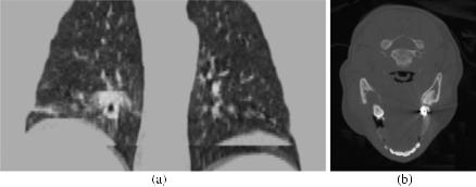
There are many artifacts that can arise in CT scanning. If very dense objects, such as metal fillings, are visible in the scan, the back-projection process will mean that these appear as streaks in the reconstructed image [37]. If there is a region of high density material, for example a thick area of skull bone, this effectively filters out lower energy X-rays and leaves a higher energy beam that is less easily absorbed. The result can be shadows beyond such regions and these are known as beam hardening artifacts. Motion can also cause significant artifacts in CT (see Fig. 11.2).

Despite the potential for artifacts and radiation dose, CT is able to produce some spectacular anatomical reconstructions (see Fig. 11.1). It is also worth noting that

Fig. 11.2 (a) Lung CT with multiple motion artifacts. There are step changes visible at various points, especially towards the bottom of the image, as the patient moves due to breathing. (b) Head CT with visible streak artifact from a filling. There are radial dark and light lines centered on the filling

CT imaging should be entirely geometrically correct—there should be no warping or distortion and the reconstruction should be an accurate reflection of the anatomy of the subject.

11.2.2 Positron Emission Tomography (PET)

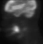
The mathematics of PET is superficially very similar to that of CT, since the signals are related to absorptions along linear trajectories. The physics is very different, however, and quite fascinating, as it involves anti-matter. There are a number of isotopes that emit positrons, including 11C, 13N, 15O and 18F. These have short half lives of only a few minutes and are not easy to produce. They require a cyclotron in close vicinity to or in the hospital and care must be taken in transporting these radioactive chemicals. These are crucial elements in organic chemistry, however, which makes it possible to image the uptake of a wide range of organic molecules. The process of producing these molecules is known as radiochemistry. The most common is Fluorodeoxyglucose (FDG), in which a OH group in glucose is replaced with 18F. This is readily used in imaging due to the relatively long half life of 18F (110 minutes) compared to 15O (2 minutes). The action of FDG within the body is very similar to glucose, in the sense that it is taken up by cells that are highly metabolizing (i.e. using energy). This includes active brain cells and also rapidly developing cancer cells. An example of a PET scan is shown in Fig. 11.3.

Having labeled a particular molecule, the radioactive marker is injected or ingested by the patient. The take-up of the radio-labeled molecule can then be imaged. As the nucleus decays, it emits a positron—the anti-matter equivalent of an electron. Within a short range, perhaps a few millimeters in tissue, this will annihilate with an electron. Two high energy (511 kEv) photons are given off at nearly 180◦. A ring of

Fig. 11.3 A sagittal section through a PET scan showing activity in the brain but also in a cancerous lesion within the mouth

highly sensitive photon detectors is used and the coincidence of two nearly simultaneous photons is considered to be a positive count, which means that there was a positron emitted somewhere along the line between the detectors. The lines forming the combinations of all sets of detectors can be organized into parallel sets at a given angle and considered as similar to tomographic projections, and methods similar to CT reconstruction can be used. Correction for attenuation is required and, for this purpose, a transmission scan similar to a CT scan is taken.

Being based on a photon counting device, the accuracy and quality of PET strongly depend on the number of events being measured. There are several effects that can impact the resolution and the SNR. These may involve physical effects (e.g. photon scattering and attenuation), counting effects (e.g. amount of injected tracer, limited photon statistics, random photon counting) and physiological effects (e.g. subject motion, tracer metabolites, tracer selectivity). For this reason, it is not possible to state a single typical number for SNR.

Due to the large number of factors that can impact PET quality, the subject of PET image reconstruction is an ongoing research field. One of the more successful range of algorithms is the use of statistical methods to provide expectation maximization. The maximum likelihood expectation maximization (ML-EM) algorithm, originally suggested by Dempster in 1977 [23] can be applied to emission tomography in a manner suggested by Shepp and Vardi [73]. An estimate of the concentration distribution of the metabolite Ij (0) is forward projected to provide a predicted set of measurements at the detectors.

This method is very time consuming and the efficiency can be significantly improved using the ordered subsets EM algorithm which uses subsets of the input voxels at each iteration [36].

11.2.2.1 Characteristics of 3D PET Data

PET is particularly suitable for imaging molecular, functional processes, but has a much lower resolution and SNR than the anatomic techniques such as MRI or CT (see Fig. 11.3). There is, in fact, a physical limit on the possible resolution of PET. This is in part due to the distance travelled by the positron before annihilation with an electron (typically a few millimeters) and also due the fact that the emitted

photons from the annihilation are not exactly at 180◦. Despite the resolution limits, PET is very useful for displaying metabolism.

11.2.3 MRI

It is often said that CT provides structural, or anatomical information, at high resolution, while PET provides ‘functional’ information. MRI is a third piece of the puzzle: it is most sensitive to hydrogen present in water and is therefore good at imaging soft tissues, as they contain a lot of water.

The principles of MRI are completely different from those of the tomographies. It is inherently 3D and where, for other modalities, ‘depth’ and ‘absorption’ play a role, this is not the case for MRI: deep lying tissues are as well visualized, often better, than superficial ones. The reason is that the scanning doesn’t happen in the actual image space but in the Fourier domain, also called ‘k-space’. It is there that different positions play a role.

The basis of MRI is the nuclear magnetic resonance (NMR) effect. This is observed for any nucleus but, in the case of medical imaging, we are almost exclusively interested in hydrogen. Since a large quantity of the body is water, which contains two hydrogen and one oxygen atoms, hydrogen is the most common atomic nucleus in the body, in fact accounting for about 63 % of the atoms in the body. In the presence of a high magnetic field, spin state of the hydrogen nucleus (in fact a single proton) is split into two energy levels: being aligned with the field, or against it.

Main Field: B0 Hence, the first ingredient of MRI is a very strong, permanent, spatially uniform, magnetic field, B0. Protons have their own magnetization, proportional to their ‘spin’. Thus they act as little magnet. When introduced in the scanner, they will tend to be parallel to this main field. In fact, they precess around it at a resonant frequency proportional to the external field: the Larmor frequency ω0. Although NMR is a quantum effect, the sum of all spins induced is a small but macroscopic magnetization for each voxel position.

RF Field: B1 A second, much smaller, field is switched on. This field is a function of time and oscillates at the frequency ω0. This means it is in resonance with the hydrogen nuclei. The plane in which B1 oscillates is chosen at an angle α from B0 (in an ideal experiment perpendicular, but in practice different ‘flip’ angles, α, are used). This excites nuclei to be aligned against the field and causes them to precess in synchrony.

Gradient Field Gt x As a result of B0 and B1, we have a small but measurable magnetization oscillating in the measurement coils in a plane transversal to the main field. By linearity, all pixels contributions add up and we end up with an oscillating magnetic field whose strength depends on the amount and environment of water molecules. In NMR or MR spectroscopy, what we would change is the resonance