Материал: [2.1] 3D Imaging, Analysis and Applications-Springer-Verlag London (2012)

frequency, to investigate different types of molecules. In MRI, we want images. Thus the resonant frequency stays similar, but the main field is modified by the addition of a linearly varying field. This makes the resonance frequency linear in position, in direction ‘x’. Each pixel or voxel now contributes with a slightly different frequency. Before applying this gradient, another perpendicular gradient is applied in the third direction, for a short while. This makes spins precess faster in that direction for a short while, thus when this ‘phase-encode’ gradient is switched, they get back to their previous frequency of rotation, but with an additional dephasing proportional to their ‘y’-coordinate. Thus, when we ‘read’ the magnetization, what we read is the contribution from each pixel, but weighted by a term dependent on position, and the gradients applied. It is not too hard to see that this term can be written e−ikx x+ky y , where k is a function of gradients and when they were switched on and off. This is the k-space often described for MRI and the measured signal corresponds to a Fourier transform. It is actually possible to excite an entire 3D volume and, for example, frequency encode the x direction and phase encode the y, z directions, although this is relatively slow.

Relaxation If left alone, the spins interact with their environment and with each other, leading to exponential decays, which are the source of the main image contrasts (T1 and T2) mentioned below.

11.2.3.1 Characteristics of the 3D MRI Data

As for CT, classical MRI is thus a 3D modality, which can be imagined as a stack of 2D slices. The most common acquisition is indeed to excite one slice at a time, and frequency encode and phase encode in two directions in that plane. MRI can be acquired directly as a full 3D volume. This means phase-encoding two directions. It is possible to have non-standard, non-lattice acquisition patterns, such as radial, spiral and rose-like. Modern advances in reconstruction theory have led to the use of different types of random sampling patterns.

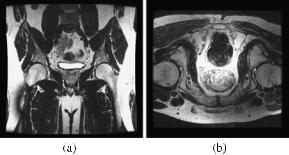
Image Quality and Artifacts The most typical artifacts for MR acquisition are ‘Nyquist’ artifacts, also known as ‘aliasing’ artifacts, which are artifacts related to a spatial sampling rate that is too low. 3D MR acquisitions can be particularly affected by them. In particular, Gibbs ringing artifacts are frequent near edges. These are due to unavoidable truncations in the acquisition. Further to this, the contrast of the image is determined by the center of the k-space. It can happen that outer parts are then undersampled, leading to blurred images. The phase encode direction is the slowest to acquire. So, to make scans faster, this direction may be undersampled. This can lead to foldover or wrap-around artifacts, where parts of the image which are out of the field-of-view seem to fold inside it. Related motion artifacts are also more visible in this direction. Examples of MRI artifacts are shown in Fig. 11.4.

Apart from the main magnetic field, all fields change with time. This creates eddy currents, which induce fields and thus distort the picture. The typical artifact

Fig. 11.4 Examples of MRI artifacts—(a) aliasing causing wrap-around near the sides of the image and (b) intensity inhomogeneity (brightness at the center) and ringing (wave-like patterns inside dark prostate region) in an image taken with a transrectal coil

due to such eddy currents is a distortion, possibly affine (shear, etc.). See Erasmus et al. [27] for further reading on MRI artifacts.

A different type of artifact can arise due to the main field being non-uniform or the gradients not being perfectly linear functions. Such inhomogeneities lead to spatial distortions of the image. There are also local imperfections of the magnetic field due to local changes in magnetic susceptibility. These artifacts lead to non-affine, localized distortions at interfaces; for example, tissue-air. So, unlike CT, it cannot be guaranteed that MRI is a geometrically correct representation of the patient.

Resolution δx is inversely proportional to the width in k-space, δx 1/ k. Small voxels are also noisier, thus there is always a trade-off between resolution and other desirable qualities of the image, such as SNR. This again is something that can be decided by operators, thus might be influenced by the application. Typical resolutions for human, in vivo MRI, are between 1 mm and 2 mm, with typical image sizes between 128 × 128 to 256 × 256.

MR images are, from the Fourier transform reconstruction, complex by nature, with the magnitudes of the complex numbers being used to display the image. Although noise in MRI is Gaussian, provided we consider their complex form, the noise on the displayed magnitudes is Rician. It is important for the computer scientists performing post-processing operations to keep this in mind.

Standard MR modalities have sufficient SNR that the noise can be approximated as Gaussian (with some correction factors) but for some other techniques, such as diffusion MRI (see Sect. 11.6), this is usually not true. We refer the reader to Rajan et al. [66] for more details on SNR in MRI.

Note that there are always trade-offs. With longer scan times, we can improve SNR at the risk of augmenting sensitivity to motion.

Contrasts: There is a wealth of different contrast weighting in MRI, thus, for a specific 3D application, it is nearly always useful to discuss the requirements with MR physicists, as it is often possible to tune the scan. However, one should keep in mind that, in most cases, these contrasts are not mutually exclusive. Images are weighted more towards one type of property, but always contain some element of the other.

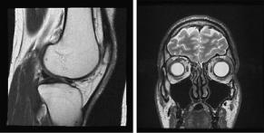
The simplest contrast conceptually is the proton density scan, but this has few clinical applications. Typical clinical images are ‘T1’ or ‘T2’-weighted, which means that the contrast is a relaxation rate relating to the spin-lattice or spin-spin

Fig. 11.5 Example MRI images: a T1 image of the knee (left) and a T2 image of the head (right)

interactions. Examples of such images are given in Fig. 11.5. It is also possible to use phase contrast (remember the complex number nature of the data), to visualize flows and even tensor contrast in diffusion tensor MRI (see Sect. 11.6).

11.2.4 Summary

For the three modalities that we have considered, this section has tried to underline where artifacts come from and what kind of 3D data to expect. In summary, CT is good for very high quality 3D images of specific regions focussing on bone and other dense tissues. MRI is the method of choice for visualization of soft tissue and is very flexible, but is slightly lower resolution than CT and more sensitive to motion. PET is lower resolution again, but provides functional data, since it shows where metabolism is occurring. Another message is that some knowledge of signal processing is a vital skill for understanding why medical images look as they do, in particular issues relating to the Nyquist-Shannon sampling theorem. Note that recent developments in reconstruction for all modalities are tending towards iterative reconstruction methods. This is the default in PET and there are algebraic methods in CT and conjugate gradient methods in MRI. So basic knowledge of inverse problems and numerical linear algebra can also be helpful. We haven’t covered ultrasound due to lack of space and also because it is less commonly used in a 3D modality.

11.3 Surface Extraction and Volumetric Visualization

As previously mentioned, much of this book concentrates on 2D surfaces embedded in 3D space. Although medical images are volumetric 3D representations of the patient, there are times when such a surface representation is useful. For example, triangulated surfaces are readily rendered by graphics hardware. A surface representation would be useful to provide an interactive 3D model of the patient. In this section, we will consider how such a representation can be created from a volume image, but also consider ways that a volume image can be rendered without extracting a surface.

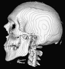
Fig. 11.8 A skull surface extracted from a CT image showing typical staircase artifacts. These can be reduced by smoothing the surface or by blurring the 3D image before applying marching cubes. This latter approach is often better

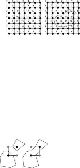
(the corners of a cube). This could provide 256 potential cases, but by adjusting for rotational and other symmetries these can be reduced to 15 cases. Ambiguities in 3D, if not dealt with correctly, can lead to holes in the resulting surface. There are a number of possible solutions to this, for example using tetrahedra rather than cubes.

Volumetric medical images usually do not have resolutions of comparable quality to what is achieved with range data. Partly as a consequence of this, surface extraction algorithms such as marching cubes [47] may produce surfaces with typical ‘staircase’ effects. Further processing may smooth the surface or decimate it. It is often better to smooth the 3D volume before running marching cubes as this reduces the noise in the dataset. As mentioned above, the triangulation can contain singularities (zero angled triangles), holes, duplicate triangles, folds and so on, if the implementation is not robust.

Example: Curvatures and Geometric Tools Once the surface has been extracted, different operations are possible for medical imaging applications. We will illustrate briefly with the example of curvatures. Curvatures are an intuitive quantity but, since they involve second derivatives, they tend to be very sensitive to surface irregularities [6, 7] They can be used as a quantification of the surface or as a tool to evolve the surface [5]. Figure 11.9 shows some illustrative examples.

11.3.2 Volume Rendering

It is also possible to produce a rendering of the anatomy from a model without extracting a surface first. This method is known as volume rendering. The idea originated in computer graphics before its application to medical imaging, but this method is ideally suited to rendering of volumetric data such as CT or MRI scans. A volume rendering of a CT image is shown in Fig. 11.10. The idea is very similar to