Материал: Крючков Фундаменталс оф Нуцлеар Материалс Пхысицал Протецтион 2011
Poisson distribution approximates hypergeometrical and binomial when pN → ∞; n → ∞; p → 0 given рп has the finite limit рп = λ. This approximation is normally used if р < 0,1.
The mathematical expectation and the variance for a random quantity distributed by Poisson’s law coincide and are equal to the value of the parameter λ = рп.
Normally distributed random quantities
Most of the experimentally obtained, measured or observed continuous random quantities are distributed by normal law:
ϕn (x) = |
1 |
|
|
− |
(x − a)2 |
|
|||
|
|
|
exp |
|
|
. |
(4.24) |
||
|
|
|
|
2 |
|||||
|
|
|
|||||||
|
σ 2π |
|
|
|
2σ |
|
|
||
|
|
|
|
|
|
|
|||
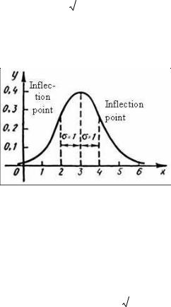
The quantities σ and а are normal distribution parameters. The plot for this distribution is a normal curve or a Gaussian (Fig. 4.2).
Fig. 4.2. Normal curve
A normal curve with the parameters а = 0 and σ = 1 is called standard. The function ϕn (x) has the following properties:
∙it exists at all actual values of the argument;
∙ has the extreme point at х = а, ϕn |
(а) = |
|
1 |
|
; |
|
|
|
|
|
|||
σ |
|
2π |
||||
|
|
|
|
|
||
∙is symmetrical about the axis through х = а;
166
∙has two knee points, left and right of х = а with abscissas, respectively,
x= a − σ and x = a + σ .
It is easy to verify that normal distribution parameters have the meaning of the mathematical expectation and the RMS deviation:
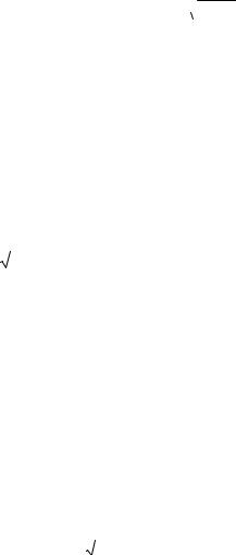
a = M(X) и σ = 
 D( X ) .
It can be shown that normal curves with coinciding σ are identically shaped and differ just in the maximum coordinate shift. The value of the variance, and more exactly, σ (RMSD), influences greatly the normal curve shape. With a decrease of σ, the curve tends to become “narrower”, extends upwards and gets needle-like; if σ increases, the curve lowers, gets “wider” and approaches the abscissa axis.
If a random quantity Х is distributed normally, then
P(x < X < x |
) = 0,5 × |
|
x - a |
|||
|
Ф |
1 |
||||
σ |
||||||
1 |
2 |
|
|
|||
|
|
|
|
|||
|
x |
2 |
- a |
|
|
||
|
- Ф |
|
|
|
, |
(4.25) |
|
|
σ |
||||||
|
|
|
|
|
|||
|
|
|
2 |
|
x |
|
t 2 |
||
where |
Ф(x) = |
|
|
|
∫exp − |
|
dt is the integral of the probabilities, the |
||
|
|
|
|
||||||
2π |
2 |
||||||||
|
|
|
0 |
|
|
||||
values thereof being tabulated.
The formula (4.25) is simplified if the interval limits are symmetrical about the mathematical expectation:
|
|
|
|
|
|
|
|
|
|
|
|
||||
P( |
|
X − a |
|
≤ )= Ф |
|
. |
(4.26) |
|
|
σ |
|||||
|
|
|
Lognormal distribution
A continuous random quantity Х has a lognormal distribution if its logarithm obeys to normal law. The probability density for lognormal distribution is:
ϕ (x) = |
|
1 |
|
|
− |
(ln x − ln a) |
2 |
|
|
||
|
|
exp |
|
. |
(4.27) |
||||||
|
|
|
|
|
|
||||||
|
σ |
|
2π x |
|
|
2σ |
2 |
|
|
|
|
|
|
|
|
|
|
|
|
||||
It can be proved that numerical characteristics of a lognormally distributed random quantity have the following form:
167
M (X ) = a exp(σ 2 / 2), Me(X ) = a,
(4.28)
D(X ) = a2 exp(σ 2 )(exp(σ 2 ) −1).
Lognormal distribution is rather commonly used to describe a distribution of profits, a distribution of impurities in alloys and minerals, the longevity of products in wear and aging conditions and so on.
Distributions relating to normal distribution
In mathematical statistics, the most common distributions are χ 2 (Pearson), t (Student) and F (Fisher) distributions. All these distributions relate to normal distribution. In turn, common use of normal distribution is determined, as we will see, exclusively by the central limit theorem (CLT) (see Section 4.6). Due to being specially important, all above-mentioned distributions are tabulated and contained in various manuals and reference books [3].
Hereinbelow, we have introduced one-dimensional standard normal distribution as a distribution with the mathematical expectation а = 0 and
the variance σ 2 = 1, its density being
ϕ (x) = Ф'(x) = |
|
1 |
|
− |
x2 |
|
|
|
|
|
|
e 2 . |
(4.29) |
||||
|
|
|
||||||
2π |
||||||||
|
|
|
|
|
|
|
||
In a general case, one-dimensional normal distribution is characterized
by the mathematical expectation а and the variance σ 2 . Then, any onedimensional normal distribution can be treated as a distribution of a random quantity:
η = a + ξ 
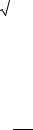
 σ 2 ,
σ 2 ,
where the random quantity ξ obeys to standard normal law.
Pearson distribution. Let ξ1,...,ξn be independent random quantities distributed by standard normal law. The distribution of the random quantity:
χ 2 = ξ12 + ... + ξn2
168

is called χ 2 –distribution (Pearson distribution) with п degrees of freedom.
χ 2 –distribution has the density
|
|
|
1 |
|
|
|
n |
−1 |
− |
x |
|
|
h(x) = H '(x) = |
|
|
|
|
|
x 2 |
|
e 2 (x > 0) , |
(4.30) |
|||
|
n |
n |
|
|
||||||||
|
|
|
|
|
|
|
|
|||||
|
|
|
|
|
|
|
|
|||||
|
2 2 |
|
|
|
|
|
||||||
|
Г |
|
|
|
|
|
|
|
||||
|
|
|
|
|
|
|
||||||
|
|
|
2 |
|
|
|
|
|
|
|||
where Г(n) is a gamma function. |
|
|
|
|
|
|
|
|
||||
Further, the following property will be useful to us. Let |
ξ1,...,ξn be |
|||||||||||
independent normally distributed random quantities with the identical parameters а and σ 2 . We shall assume that
η= 1 (ξ1 + ... + ξn ) . n
Then the random quantity
χ 2 = |
1 |
[(ξ1 −η)2 + ... + (ξn −η)2 ] |
(4.31) |
|
σ 2 |
||||
|
|
|
has the χ 2 – distribution but with п– 1 degrees of freedom.
There is one more interpretation (case) of Pearson distribution. Let п independent tests be conducted (polynomial case or Bernoulli case), in each of which one of the events Аi (I = 1,…, L) may occur with the probability рi. Let us denote the number of the occurrences of the event Аi by тi. Then it follows from the multidimensional analog of the Moivre-Laplace integral theorem that the random quantity:
χ 2 = |
(m − np ) |
2 |
+ ... + |
(m |
L |
− np |
L |
)2 |
|
|
1 |
1 |
|
|
|
|
, |
||||
np1 |
|
|
|
|
npL |
|
|
|||
|
|
|
|
|
|
|
|
|
||
with n → ∞ , is asymptomatically distributed by χ 2 |
law with L – 1 degrees |
|||||||||
of freedom. |
|
|
|
|
|
|
|
|
|
|
t–distribution. Let ξ and χ 2 |
be independent random quantities, ξ being |
|||||||||
distributed by standard normal law, and χ 2 having a Pearson distribution
169
with п |
degrees of freedom. The distribution |
of |
the |
random |
quantity |
||||||||||||||||
τ = ξ / |
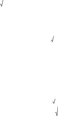
χ 2 / n |
is called a t–distribution with |
п degrees of freedom (Student |
||||||||||||||||||
distribution). |
|
|
|
|
|
|
|
|
|
|
|
|
|
|
|
|
|
|
|
||
This distribution has the density |
|
|
|
|
|
|
|
|
|
|
|
|
|
|
|
|
|
|
|
||
|
|
|
|
|
|
|
n + 1 |
|
|
|
|
|
|
− |
n+1 |
|
|
||||
|
|
|
1 |
|
|
Г |
|
|
|
|
|
|
|
x |
2 |
|
|
|
|||
|
|
|
|
|
2 |
|
|
|
|
||||||||||||
|
|
|
|
|
|
|
|
|
|
2 |
|
|
|||||||||
|
|
t(x) = T '(x) = |
|
|
|
|
|
|
|
|
|
|
1 + |
|
|
|
, |
(4.32) |
|||
|
|
|
|
|
|
|
|
|
|
|
|
|
|
||||||||
|
|
|
π n |
|
|
|
n |
|
|
|
n |
|
|
|
|
|
|||||
|
|
|
|
|
|
|
|
|
|
|
|
|
|
||||||||
|
|
|
|
|
|
|
Г |
|
|
|
|
|
|
|
|
|
|
|
|
||
|
|
|
|
|
|
2 |
|
|
|
|
|
|
|
|
|
|
|||||
where Г(т) is the gamma function.
Let ξ1,...,ξn be independent random quantities similarly distributed by normal law with the average а. Let us assume that
η = |
1 |
(ξ1 + ... + ξn ) , ς = (ξ1 −η)2 + ... + (ξn −η)2 . |
||||||||
|
||||||||||
|
n |
|
|
|
|
|
|
|
|
|
Then the random quantities ζ è η |
are independent and the random |
|||||||||
quantity |
|
|
|
|
|
|
|
|
|
|
|
|
|
|
|
|
(η − a) |
||||
|
|
|
τ = |
|
n |
|||||
|
|
|
|
|
|
|
|
|
|
|
|
|
|
|
|
|
|
|
|
|
|
|
|
|
|
|
ς |
|||||
|
|
|
|
|
|
|
||||
|
|
|
|
|
|
|
n −1 |
|
|
|
has a t–distribution with п – |
1 degrees of freedom. |
|||||||||
F–distribution |
relates to Pearson distribution as follows. Let χ12 , χ22 be |
|||||||||
two independent |
random |
quantities |
having an χ 2 distribution with |
|||||||
n1 and n2 degrees of freedom respectively. The distribution of the random quantity
|
ϖ = |
n2χ12 |
|
|
n1χ22 |
||
|
|
||
is |
referred to as F– distribution (Fisher distribution) with the parameters |
||
n1 |
and n2 . The density of the F–distribution is: |
||
170