Материал: Крючков Фундаменталс оф Нуцлеар Материалс Пхысицал Протецтион 2011

error. And, vice versa, if the weight values observed at a measurement point turn out to have an error in excess of the level desired, a special study is required to find out why this has happened. And such a study needs at least some of the above-mentioned error sources to be identified, and individual contributions thereof to the error estimated. By a “special study” we mean, say, calibration.

Models of errors

We have discussed just some of many error sources. Though it is their cumulative effect that we are interested in the most, it is often convenient or even necessary to form a reasonable mathematical model to identify errors as such and find out how these are interlinked. Therefore, a model helps combine errors correctly, find their cumulative effect and identify sources of errors, and provides safeguards against potential skips of certain sources. Let us discuss this in more details and introduce two basic models: an additive model and a nonadditive (so-called multiplicative) model of error.

Additive model. This is the simplest model (4.40) we have already made use of. Despite being simple, additive models are often used in practical activities and, in many instances, give a nearly real result. A note should be made that any model is a mathematical description of reality. Experience shows that humans tend to employ simpler models in practice, occasionally even at a sacrifice of detailed and adequate description of reality. Simple models are therefore commonly used.

Let, say, хbe the measured gross weight value of a container with UO2

powder, g; μ the true value of this quantity, and ε the error, so then х= μ + ε .

Therefore, if summed up, the true value and the error would give the measured value. If measurements are done on standard samples of the known weight μ with their measured value хrecorded, then the distribution function ε can be constructed based on the measurements.

Multiplicative model. Describing a measurement result by a simple sum of the true value and the errors often gives an acceptable description of the real situation, though not altogether universally. If the absolute error of measurement grows with the measured value, the so-called multiplicative model is employed.

Assume that у is the measured value of the uranium concentration in UO2, α is the true quantity and η is the measurement error.

186

Then у= α + η. Let us be interested in the net weight of uranium in the container from the previous instance rather than in the weight of oxide. By multiplying х by у, we get ху = μα + μη + αε + εη, which no longer makes a simple additive model.

In this case, it will be more convenient to use a multiplicative model:

x = μ (1+ε), у= α (1+η).

Then the expression for the uranium weight will look as follows: ху= μα (1+η)(1+ε).The latter expression is apparently much simpler, more graphic and more convenient in terms of error estimates. So, though additive models are frequently convenient to use, one should avoid using these in all cases as the net effect of several errors is not always a simple sum thereof.

Estimation of NM measurement errors

Confident estimates of nuclear material measurement errors are required to estimate the significance of the inventory differences detected. These estimates depend on the models adopted to calculate errors and interpret «random» and «systematic» errors.

Test measurement data is expected to satisfy to accuracy and precision requirements. Precision is characterized by repeatability and reproducibility of measurement data.

Repeatability is determined by the variance (spread) of the data obtained by one operator when measuring one sample in similar conditions. Reproducibility is determined by the variance of the measurement data for a sample measured by more than one operator for several days in various conditions.

Accuracy of data depends on the quantity of the systematic measurement error. The systematic quantity error can be estimated as the average difference (in the sense of mathematical expectation) between the values measured and the true value (4.40). A small quantity of the systematic error in data is equivalent to a high accuracy thereof.

Basic principles of measurement error calculations:

1)the total measurement data errors are computed as the sum of the random error and the systematic error as reduced to the same confidential probability;

2)the values of all errors are normally reduced to the confidential probability of 0.95;

187

3)when computing the random error in data, one should treat the respective quantities as normally distributed;

4)one should consider the systematic error of a measurement result on the assumption of uniform (equally probable) law of distribution of constituent quantities.

Agreed notation.

1. According to GOST State Standards, the following designations should be used to denote errors of the quantity х as reduced to the confidential probability of 0.95: random error – S(x), systematic error – θ (x), total error – δ (x).

2.When choosing the confidence probability рother than equal to 0.95, one should use the record рS(x), рθ (x), рδ (x).

3.The absolute measurement error should be designated as DS, Dθ , D.

4.The ultimate measurement result should be presented as х= Х, δ =… %, θ =… %, р = 0,95, where Х is the root-mean-square value of the measured quantity х, and θ is the maximum boundary of the nonexceptional residue for the systematic error of the quantity хunder determination.

Direct measurements

1. Estimation of the result with a large number (n > 3) of measurements for the quantity х:

188

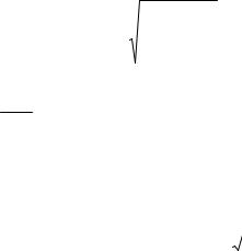
where рS(x) = pts×S(x) is the factor of reduction to the confidential probability P, Student’s coefficient (Table 4.2), [3] and [8].

2. Estimation of the result with single measurements of the quantity х (n≤3). Single measurements of the quantity х should be preceded by a metrological test of the instrument to be used. Such test involves multiple (N > 20) measures of a certain quantity a similar to the quantity х, and determination of σ for the obtained value set аi:

∑ai

where A = i =1 .

N

In further measurements of the quantity х, the result is estimated as follows:

189

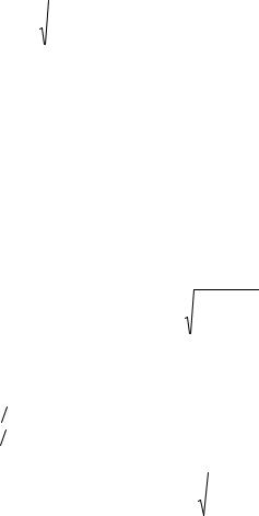
where Kσ is the coefficient that allows for various statistical significances of results when the instrument is tested and the quantity хis measured

results when the instrument is tested and хis determined

Indirect measurements

1. Estimation of the result in measuring the quantity y = f (x1, x2,…, xn) in a single experiment:

·the input is measured values xi, as well as the random error and the systematic error of the constituent quantities S(xk) and θ (xk);

·the errors of the constituent quantities that are part of the formula to determine the quantity у, but not measured in the given experiment

(constants, coefficients, certification results) shall be treated as θ (xk);

·the result Y is estimated by the following formula:

Y = y,

The total measurement data error is δ (Y) = S(Y)+θ (Y).

Often either S(Y)>>θ (Y) or θ (Y)>>S(Y). In these cases, the error calculation formula becomes simpler.

2. Estimation of the measurement result for the quantity y = f (x1, x2, …, xn) in a multiple experiment:

190