Материал: Маслов ИНТРОДУЦТИОН ТО ПХЫСИЦС ОФ СЕЦОНД-ОРДЕР МАГНЕТИЦ 2015

Скачать файл

Заказать новую работу

Внимание! Если размещение файла нарушает Ваши авторские права, то обязательно сообщите нам

C. At T →0 (T θ) the order parameter is

≈1− 2e−2

x2 ≈1− 4e−2

In this case

NµB2

4e−2

NµB2 4e−2

χ =

≈

T −θ

−2

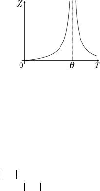
Thus the magnetic susceptibility exponentially tends to zero at T →0. The resulting temperature dependence of χ is shown on Fig. 21.1.

Fig. 21.1. Temperature dependence of ferromagnet magnetic susceptibility

Why is the magnetic susceptibility tend to zero at T →0 and at T →∞ ? The reason is that in both cases it is nothing to ordering: at T →0 all the magnetic moments are already ordered (even without a magnetic field), and at T →∞ atoms do not have the mean magnetic moments.

22. Critical exponents

We obtained that at T → θ the magnetic susceptibility diverged by the law χ(T )− T −θ−1 (see § 21), and order parameter has the squareroot singularity ∆(T )− T −θ1/2 at T → θ− (see § 19). As for heat ca-

pacity, in the mean-field approximation it has the abrupt			jump (see
§ 20). Critical exponents α , β and γ are denoted as follows
C (T )−	T −θ	−α ;

∆(T )−(T −θ)β ;			(22.1)
χ(T )−	T −θ	−γ .

In the case of ferromagnetic phase transition in the mean-field approximation we have α = 0 , β = 12 and γ =1. Let us compare these results

with the numerical calculations (3D Ising model) and experimental data (see Table 22.1).

Table 22.1

Critical exponents obtained using mean-field approximation and numerical calculations along with experimental data

Critical exponent	Mean-field	Numerical	Experiment
Critical exponent	approximation	calculations	Experiment
	approximation	calculations
α	0	0,12	≈ 0,1

β	0,5	0,31	0,3 ÷0,4

γ	1	1,25	1,2 ÷1,4

α + 2β + γ	2	1,99	1,9 ÷2,3

Overall, there are about ten different critical exponents, but some of them depend on each other. It can be exactly shown that (see Table 22.1)

α + 2β+ γ = 2 .

(22.2)

In the mean-field approximation the expression mentioned above is also correct, but unfortunately each exponent separately is incorrect.

23. Exact solution of the Ising model in one dimension

Recall that the	Curie temperature, by definition, is
θ = ∑J (Rl )= zJ, where	z is the number of nearest neighbors of each
Rl ≠0

atom. In the formula for θ we denote the J (Rl )= J > 0 for the nearest

neighbors and consider the J (Rl )= 0 for other atoms. Therefore, for

the one-dimensional chain of magnetic moments the mean-field approximation predicts the ferromagnetic phase transition at θ = 2J (if the interactions between only nearest neighbors are taken into account). Let us solve the problem for one-dimensional chain of magnetic moments with interactions only between the nearest neighbors exactly. The Hamiltonian in the Ising model is

				= −	1	∑	/				(23.1)
			H	= −		∑		Jij σiz σjz		− h∑σiz ,	(23.1)
					2 i, j					i

	µiz	,	h = µB H , and					σiz	= ±1 are the eigenvalues of opera-
where σiz =	µB	,	h = µB H , and					σiz	= ±1 are the eigenvalues of opera-
	µB

tors σiz . Note again that the interaction occurs only between the nearest neighbors, so, Jij = J > 0 if i and j are the numbers of the nearest mag-

netic moments and Jij = 0 otherwise. Let us numerate all the magnetic

moments in the system from “1” to “N”. Therefore the Hamiltonian takes the form

		(23.2)
H	= −J σ1z σ2z − J σ2z σ3z −... − J σN −1,z σNz − h(σ1z +... + σNz ).	(23.2)
Since	N 1 the boundary conditions are not essential. Let us make

them periodical, i.e., “close the chain into the ring”. In other words, we add into the Hamiltonian between the 1-st and N-th magnetic moments

the following term			−J
the following term			−J	σNz σ1z . Next, let us calculate the partition func-
	ˆ					En
	−H		∑		−	En
		=	∑	e T			, where n are the numbers of the Hamiltoni-
tion Q =Tr e	T	=		e T			, where n are the numbers of the Hamiltoni-
			n

an eigenstates and En are the corresponding energies. If we know the partition function, we can calculate the free energy F = −T lnQ , and finally – the order parameter x.

Every state “n” is defined by the set of N numbers σiz

each is equal

+1 or –1, and ∑ is the sum over all number sets {σiz }

Q = ∑

{σiz }

e− T

{σiz } .

(23.3)

{σiz }

i =1,..., N ,

The Hamiltonian

the function

operators

σiz

). Since

{σiz }

= σkz

{σiz }

k , then

= H (σ1z ,σ2z ,...,σNz

σkz

{σiz }

= H (σ1z ,σ2z ,...,σNz ){σiz } .

Therefore

Nz )

,σ

2 z

,...,σ

( 1z

e− T

{σiz } = e−

{σiz } .

Considering these expressions, for the partition function we obtain

Q = ∑

{σiz }

e−

H (σ1z ,...,σNz )

{σiz }

= ∑e−

H (σ1z ,...,σNz )

{σiz }

(23.4)

H (σ1z ,...,σNz )

= ∑ ∑

... ∑ e

−

σ1z =±1 σ2 z =±1 σNz =±1

where

H (σ1z ,...,σNz )= −Jσ1z σ2z − Jσ2z σ3z −... − JσN −1,z σNz − JσNz σ1z − −hσ1z − hσ2z −... − hσNz .

So,

Q = ∑

... ∑ exp

σ1zσ2z

σ2zσ3z +... +

σN −1,zσNz +

σ1z =±1 σNz =±1

σ2z +... +

σNzσ1z +

σ1z +

σNz

= ∑ ... ∑ exp

σ1z σ2z

(σ1z + σ2z )+

σ2z σ3z

σ1z =±1 σNz =±1

(σ2z

+ σ3z )+... +

σN −1,z σNz +

(σN −1,z + σNz )+

σNz σ1z +

(σNz + σ1z ) .

Denote the 2 ×2 matrix A

A =

(23.5)

1,1

1,−1

−1,1

−1,−1

where the matrix elements are

Aσ

,σ

= exp

σ1z σ2z +

(σ1z + σ2z ) .

2 z

Thus the matrix takes the following form

−

(23.6)

A =

e−

−

Denote the other matrix elements Aσ

2 z

,σ

,..., Aσ

,σ

in the same way.

For Q we obtain

3 z

Q = ∑ ... ∑ Aσ1z ,σ2 z

Aσ2 z ,σ3 z ,..., AσN −1,z ,σNz

AσNz ,σ1z .

(23.7)

σ1z =±1 σNz =±1

Recall the rule of matrix multiplication (A2 )kn = ∑Akm Amn . Therefore

∑ Aσ1z ,σ2 z

= (A2 )σ

Aσ2 z ,σ3 z

,σ

3 z

σ2 z =±1

∑ (A2 )σ

,σ

3 z

Aσ3 z ,σ4 z

= (A3 )σ

,σ

, …,

σ3 z =±1

4 z

∑ (AN −1 )σ

,σ

AσNz ,σ1z = (AN )σ

,σ .

σN ,z =±1

Finally, for the partition function we obtain

Q = ∑ (AN )σ

σ .

(23.8)

σ1z =±1

Источник: https://studfile.net/preview/16708691/

Смотрите также:

_1966(~1
_РГР № 1 (2)
"Логистическая технология JIT"
"Особенности правовой системы Российской Федерации" по дисциплине "Теория государства и права"
«Анализ ликвидности и платежеспособности предприятия» (на материалах ОАО Московская кондитерская фабрика «Красный Октябрь»)
«Дизайнерские дети» как профилактика инвалидизации общества
«ЗЕМЕЛЬНЫЕ РЕСУРСЫ КРАСНОДАРСКОГО КРАЯ»
«Методы учета затрат на производство продукции, работ, услуг»Курсовая работа
[2 курс] Определения
00338