Материал: Маслов ИНТРОДУЦТИОН ТО ПХЫСИЦС ОФ СЕЦОНД-ОРДЕР МАГНЕТИЦ 2015

Смотрите также:

Внимание! Если размещение файла нарушает Ваши авторские права, то обязательно сообщите нам

It is important that Jij falls off exponentially with the distance Ri − Rj between the atoms i and j, being maximum when these atoms

are nearest neighbors. This is why the so called nearest neighbor approximation is of frequent use:

Jij	J , atoms	i and	j	are nearest neighbors,	(8.19)
Jij	=				(8.19)
	0, otherwise.

For different materials the value of J varies widely, being typically in the range 0.001 ÷ 0.1 eV.

9. Interaction of two local magnetic moments

Let us explicitly express the operator ij of the pairwise interaction

energy Uij in terms of operators µi and µj of magnetic moments at at-

						1

oms i and j. Taking into account				that (Si S j )=		4µB2	(µi µj ), see
Eq. (8.2), from Eqs. (8.13) and (8.15), we have
	0	Jij

U ij =Uij −		2		(µi µj ),				(9.1)
where		2µB
where			Jij
U 0	= A −		Jij		,			(9.2)
U 0	= A −				,			(9.2)
ij		ij		2
				2

and the sign of the second term in Eq. (9.1) depends on mutual orientation of the magnetic moments since (µi µj )> 0 in the case that the spin S of two electrons at atoms i and j equals to 1 (“parallel” magnetic moments) and (µi µj )< 0 if S = 0 (“antiparallel” magnetic moments), see §

8. It follows from Eq. (9.1) that for the magnetic moments of i-th and j- th atoms it is energetically favorable to be oriented in one direction if Jij > 0 and in opposite directions if Jij < 0.

In the case that Jij > 0 for any pair of atoms (i, j) in the sample, the

total energy of the system is minimum when all magnetic moments are unidirectional. This is the ferromagnetic ordering. Next, as long as 21

Jij < 0 for any two nearest atoms and negligibly small otherwise, the total energy is minimum when any two nearest moments are oppositely directed. Such a type of ordering is referred to as antiferromagnetic. It is reminiscent of a checkerboard order. In the general case, the sign of Jij may vary with the distance between the atoms i and j, resulting in rather complex magnetic textures, neither ferromagnetic nor antiferromagnetic.

It should be pointed out that the very possibility of one or another type of magnetic order to take place in a given solid strongly depends on its crystal structure. For example, the antiferromagnetic ordering cannot occur on a triangular lattice because of frustration. Besides, in anisotropic crystals different types of magnetic order may exist along different crystal axes.

10. Heisenberg model and Ising model

Up to now we have discussed the interaction between two local

magnetic moments and derived the operator ij of the corresponding

interaction energy, see Eqs. (9.1) and (9.2). We now turn to the macroscopic system of N 1 moments. With consideration for an external

magnetic field H the Hamiltonian is

where the sum over both i and j is from 1 to N, the prime implies that

i≠ j, and we took into account that U ji =U ij . For the sake of conven-

ience let us, first, introduce the operators σi = µi µB and, second, redefine the exchange integral Jij → 2Jij in Eq. (9.1), so that

					0
								(10.2)
	U ij =Uij					− Jij (σi σj ) ,		(10.2)
and Eq. (10.1) becomes		1
		1		/
								(10.3)
H = −			∑ Jij (σi σj ) − h∑σi ,					(10.3)
		2 i, j					i

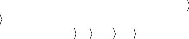
where we measured the energy from 1

∑/ Uij0 and used the designation

2 i, j

h = µB H . Note that the operators

have two eigenstates,

↑ and

σiz

↓ , with eigenvalues +1 and –1 respectively:

↑ =

↑ ,

↓ = −

↓ ,

(10.4)

σiz

see § 4.

The Hamiltonian (10.3) is referred to as the Hamiltonian of the isotropic Heisenberg model. The term “isotropic” points to equal strength of interaction between the components of magnetic moments along x, y,

and z axes: Jij (σi σj ) = Jij σix σjx + Jij σiy σjy + Jij σiz σjz . In general, how-

ever, this is not the case because of the crystal field anisotropy, and the Hamiltonian has the form

∑

Jij

H = −

σix σjx +Jij

σiy σjy + Jij

σiz σjz − h

∑σi . (10.5)

2 i, j

This the Hamiltonian of the anisotropic Heisenberg model. For the special case of Jijxx = Jijyy = Jijzz it reduces to Eq. (10.3). For another limiting

case Jijxx , Jijyy << Jijzz ≡ Jij we have the Hamiltonian of the Ising model:

		1		/
			∑					(10.6)
H = −			∑		Jij σiz σjz − h	∑σi .		(10.6)
		2 i, j				i	H = Hez , i.e.,	h = hez ,
Usually this model is simplified further taking							H = Hez , i.e.,	h = hez ,
where h = µBH:		1
	= −	1	∑	/				(10.7)
H	= −		∑		Jij σiz σjz − h∑σiz .			(10.7)
		2 i, j				i

This is the Hamiltonian we shall study in what follows.

Contrary to the case of noninteracting magnetic moments, there is now the term that accounts for interaction of moments to one another.

As before, our objective is to find magnetization M as a function of T and H.Inasmuch as H = Hez , we have M = Mez , where

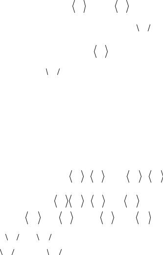
	1	N			µB	N
M =		∑	µiz	=		∑	σiz .	(10.8)
M =	V	∑	µiz	=	V	∑	σiz .	(10.8)
	V	i=1		T	V	i=1	T

Since all magnetic moments are alike, the value of σiz T does not depend on i, and hence

M =	µB N		,	(10.9)
	V	σiz T

where one can take σiz T for any one of N moments. In general this

problem has no exact analytic solution, and one must either resort to numerical calculations or make use of one or another approximation.

11. Mean-field approximation in the Ising model

As mentioned above, in the general case the exact analytic solution of Ising model with interactions can not be found. However if we repre-

sent Hamiltonian (10.7) as the sum of terms depending only on the σiz , the problem will be solved. Further we shall use the approach that make


the term σiz σjz linear in σiz .										). Conse-
Rewrite		as
Rewrite	σiz σjz	as	(σiz − σiz		+ σiz	)(σjz − σjz		+ σjz
quently								)+

	σiz	σjz	= σiz	σjz	+ σiz	(σjz − σjz			),	(11.1)
										(11.1)

	+ σjz	(σiz − σiz		)+(σiz − σiz			)(σjz − σjz

where σiz and σjz are the mean values of the magnetic moments,

σiz − σiz and σjz − σjz are the operators of magnetic moments fluc-

tuations (they define the difference between true moments and the mean value). One can see three different terms in the sum written above: terms that do not depend on fluctuations, terms that depend linearly on fluctuations, and terms that depend quadratically on fluctuations. In other words, we can present the interaction of two magnetic moments as a

sum of three types of interactions (for each pair of magnetic moments): interaction of mean magnetic moments with each other, interaction of mean magnetic moments with fluctuations, and interaction of fluctua-

tions with each other.

Let

consider

that

fluctuations

are

small,

i.e.,

)

1. Since we consider that fluctuations are

(σiz − σiz

σiz

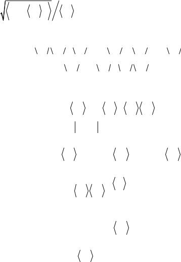
small, we neglect the terms in Hamiltonian that depend quadratically on fluctuations, but leave terms that depend linearly on fluctuations

σiz σjz ≈ σiz σjz + σiz (σjz − σjz )+ σjz (σiz − σiz )=

= σiz σjz + σjz σiz − σiz σjz .

(11.2)

This approach is called the mean-field approximation. Taking into account the approximation used (for each pair of magnetic moments) rewrite the Hamiltonian of the Ising model

	1	∑	/								(11.3)
H ≈ −		∑		Jij (σiz	σjz	+ σjz	σiz	− σiz	σjz	)− h∑σiz .	(11.3)
	2 i, j									i

Considering that Jij = J (Ri − Rj ), and consequently Jij = J ji , replacing i ↔ j , we require for the second term

∑

= ∑

(11.4)

Jij σjz

σiz

J ji σiz

σjz

Jij σiz

σjz

i, j

that is equal to the first term. The third term is a constant

∑

Jij

σz

∑

Jij ≡ E0′.

(11.5)

σiz

σjz

2 i, j

i, j

Therefore, we can write down the Hamiltonian of the Ising model in the following form

	/				(11.6)
H ≈ E0′ −∑		Jij σiz	σjz	−h∑σiz .	(11.6)
i, j				i

Considering that our system is homogeneous (i.e., it is free from intersti-

tial magnetic moments),		does not depend on j . Therefore, we
	σjz

Источник: https://studfile.net/preview/16708691/

∑ U ij − H ∑µ,

_1966(~1
"Логистическая технология JIT"
"Особенности правовой системы Российской Федерации" по дисциплине "Теория государства и права"
«Анализ ликвидности и платежеспособности предприятия» (на материалах ОАО Московская кондитерская фабрика «Красный Октябрь»)
«Дизайнерские дети» как профилактика инвалидизации общества
«ЗЕМЕЛЬНЫЕ РЕСУРСЫ КРАСНОДАРСКОГО КРАЯ»
«Методы учета затрат на производство продукции, работ, услуг»Курсовая работа
[2 курс] Определения
00438
00463