Материал: [2.1] 3D Imaging, Analysis and Applications-Springer-Verlag London (2012)
54 |
S. Se and N. Pears |
where xi,j is the image of world point Xj in image i and xˆ i,j is the predicted projection of the same world point according to Eq. (2.7) (using estimated intrinsic and extrinsic camera parameters) followed by radial distortion according to Eq. (2.6).
The vector p contains all of the free parameters within the planar projection (homography) function plus two radial distortion parameters k1 and k2 as described in Sect. 2.3.3. Initial estimates of these radial distortion parameters can be set to zero. LM iteratively updates all parameters according to the equation:
pk+1 = pk + δpk
δpk = − JT J + λJ diag JT J −1JT e,
where J is the Jacobian matrix containing the first derivatives of the residual e with respect to each of the camera parameters.
Thus computation of the Jacobian is central to LM minimization. This can be done either numerically or with a custom routine, if analytical expressions for the Jacobian entries are known. In the numerical approach, each parameter is incremented and the function to be minimized (the least squares error function in this case) is computed and divided by the increment, which should be the maximum of 10−6 and 10−4 × |pi |, where pi is some current parameter value [21]. In the case of providing a custom Jacobian function, the expressions are long and complicated in the case of camera calibration, and so the use of a symbolic mathematics package can help reduce human error in constructing the partial differentials.
Note that there are LM implementations available on many platforms, for example in MATLAB’s optimization toolbox, or the C/C++ levmar package. A detailed discussion of iterative estimation methods including LM is given in Appendix 6 of Hartley and Zisserman’s book [21].
2.4.4 Calibration of a Stereo Rig
It is common practice to choose the optical center of one camera to be the origin of a stereo camera’s 3D coordinate system. (The midpoint of the stereo baseline, which connects the two optical centers is also occasionally used.) Then, the relative rigid location of cameras, [R, t], within this frame, along with both sets of intrinsic parameters, is required to generate a pair of projection matrices and hence a pair of 3D rays from corresponding image points that intersect at their common scene point.
The previous two subsections show how we can calculate the intrinsic parameters for any single camera. If we have a stereo pair, which is our primary interest, then we would compute a pair of intrinsic parameter matrices, one for the left camera and one for the right. In most cases, the two cameras are the same model and hence we would expect the two intrinsic parameter matrices to be very similar.
Also, we note that, for each chessboard position, two sets of extrinsic parameters, [R, t], are generated, one for the left camera’s position relative to the calibration plane and one for the right. Clearly, each left-right pair of extrinsic parameters

2 Passive 3D Imaging |
55 |
should have approximately9 the same relationship, which is due to the fixed rigid rotation and translation of one camera relative to another in the stereo rig.
Once two sets of intrinsic parameters and one set of extrinsic parameters encoding the relative rigid pose of one camera relative to another has been computed, the results are often refined in a global stereo optimization procedure, again using the Levenberg-Marquardt approach. To reduce n sets of relative extrinsic parameters to one set, we could choose the set associated with the closest calibration plane or compute some form of robust average.
All parameter estimates, both intrinsic and extrinsic, can be improved if the LM optimization is now performed over a minimal set of parameters, since the extrinsic parameters are reduced from 12 (two rotations and two translations) to 6 (one rotation and one translation) per calibration grid location. This approach ensures global rigidity of the stereo rig going from left to right camera. An implementation of global stereo optimization to refine stereo camera parameters is given in the Caltech camera calibration toolbox for MATLAB [9].
2.5 Two-View Geometry
3D reconstruction from an image pair must solve two problems: the correspondence problem and the reconstruction problem.
•Correspondence problem. For a point x in the left image, which is the corresponding point x in the right image, where x and x are images of the same physical scene point X?
•Reconstruction problem. Given two corresponding points x and x , how do we compute the 3D coordinates of scene point X?
Of these problems the correspondence problem is significantly more difficult as it is a search problem whereas, for a stereo camera of known calibration, reconstruction to recover the 3D measurements is a simple geometric mechanism. Since we have sets of three unique points, (x, x , X), this mechanism is called triangulation (not to be confused with surface mesh triangulation, described in Chap. 4).
This section is designed to give the reader a good general grounding in two-view geometry and estimation of the key two-view geometric relations that can be useful even when extrinsic or intrinsic camera calibration information is not available.10 As long as the concept of epipolar geometry is well understood, the remaining main sections of this chapter can be followed easily.
9‘Approximately’, because of noise in the imaged corner positions supplied to the calibration process.
10Extrinsic parameters are always not known in a structure from motion problem, they are part of what we are trying to solve for. Intrinsic parameters may or may not be known, depending on the application.

56 |
S. Se and N. Pears |
2.5.1 Epipolar Geometry |
|
Epipolar geometry establishes the relationship between two camera views. When we have calibrated cameras and we are dealing with metric image coordinates, it is dependent only on the relative pose between the cameras. When we have uncalibrated cameras and we are dealing with pixel-based image coordinates, it is additionally dependent on the cameras’ intrinsic parameters, however, it is independent of the scene.
Once the epipolar geometry is known, for any image point in one image, we know that its corresponding point (its match) in the other image, must lie on a line, which is known as the epipolar line associated with the original point. This epipolar constraint greatly reduces the correspondence problem from a 2D search over the whole image to a 1D search along the epipolar line only, and hence reduces computational cost and ambiguities.
The discussion here is limited to two-view geometry only. A similar constraint called the trifocal tensor is applicable for three views, but is outside the scope of this chapter. For further information on the trifocal tensor and n-view geometries, please refer to [21].
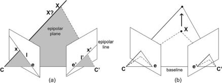
As shown in Fig. 2.7(a), the image points x and x , world point X and the camera centers are co-planar and this plane is called the epipolar plane, which is shaded in the figure. If we only know x, how is the corresponding point x constrained? The line l is the intersection of the epipolar plane with the second image plane. l is called the epipolar line, which is the image in the second view of the ray backprojected from x. As the point x lies on l , the correspondences search does not need to cover the entire image but can be restricted only to the line l . In fact, if any point on epipolar line l has a corresponding point in the second image, it must lie on epipolar line l and vice-versa. Thus l and l are called conjugate epipolar lines.
The epipole is the point of intersection of the line joining the camera centers with the image plane. The epipole e is the projection of the second camera center on the first image, while the epipole e is the projection of the first camera center on the second image.
In essence, two-view epipolar geometry describes the intersection of the image planes with the pencil of planes having the baseline as the pencil axis, as illustrated in Fig. 2.7(b). Note that the baseline is the line joining the two camera centers.11 All epipolar lines intersect at the epipole of the respective image to give a pencil of epipolar lines in each image. Note that the epipoles are not necessarily within the boundaries of the image. A special case is when the cameras are oriented in the same direction and they are separated by a translation parallel to both image planes. In this case, the epipoles are at infinity and the epipolar lines are parallel. Furthermore, if the translation is in the X direction only and the cameras have the same intrinsic parameters, the conjugate epipolar lines lie on the same image rows. This is an ideal set up when we search for correspondences between the two images. However, we
11The length of the baseline is the magnitude of the extrinsic translation vector, t.
2 Passive 3D Imaging |
57 |
Fig. 2.7 (a) The epipolar geometry establishes the relationship between the two camera views. (b) The epipolar planes rotate around the baseline and all epipolar lines intersect at the epipole
may prefer some camera vergence to improve the field-of-view overlap between the two cameras and, in this case, the images need to be warped so that the epipolar lines become horizontal again. This rectification process is discussed later in the chapter.
The epipolar constraint can be represented algebraically by a 3 × 3 matrix called the fundamental matrix (F), when we are dealing with raw pixel coordinates, and by the essential matrix (E) when the intrinsic parameters of the cameras are known and we are dealing with metrically expressed coordinates (e.g. millimeters) in the image plane.
2.5.2 Essential and Fundamental Matrices
Both the essential and fundamental matrices derive from a simple co-planarity constraint. For simplicity it is best to look at the epipolar relation using the essential matrix first and then adapt it using the camera intrinsic parameters to obtain a relation for pixel-based image coordinates, which involves the fundamental matrix.
Referring to Fig. 2.8, we have a world point X that projects to points xc and xc in the image planes. These image plane points are expressed as 3-vectors, so that they are effectively the 3D positions of the imaged points expressed metrically in their own camera frame, hence the subscript c. (Note also that they can be regarded as normalized homogeneous image coordinates, with the scale set to the focal length, f , although any non-zero scale would suffice.) We know that the three vectors Cxc , C xc and t are co-planar, so we can choose one of the two camera frames to express this co-planarity, using the scalar triple product. If we choose the right frame (primed), then we must rotate vector Cxc using rotation matrix R, to give:
xcT (t × Rxc ) = 0.
Expressing the cross product with t by the multiplication with the skew-symmetric matrix [t]x , we have:
xc [t]x Rxc = 0,
58 |
S. Se and N. Pears |
Fig. 2.8 The essential matrix E = [t]x R encodes the epipolar geometry. It is used to relate the correspondences xc and xc between two images, when these image locations are expressed in metric units. If pixel-based coordinates are used (for example, if intrinsic camera parameters are unknown) epipolar geometry is encoded by the fundamental matrix F
where |
|
|
|
|
|
|
|
|
t |
|
|
0 |
−tz |
ty |
|
||
x |
= |
tz |
0 |
|
−tx |
|
||
[ ] |
|
− |
ty |
tx |
|
0 |
||
and thus we have: |
|
|
|
|
|
|
|
|
|
|
|
|
|
|
|
|
|
and |
|
|
E = [t]x R |
|
(2.15) |
|||
|
|
|
|
= |
|
|
|
|
|
|
|
c |
|
0. |
|
(2.16) |
|
|
|
x T Exc |
|
|
||||
Thus the essential matrix encapsulates only extrinsic parameters, namely, the rotation and translation associated with the relative pose of the two cameras. The implication of this is that, in applications where R and t have not been computed in a calibration procedure, they may be recoverable from an estimate of E, which will be discussed further in Sect. 2.8.2 in the context of structure from motion.
In many practical situations, we also need to deal with uncalibrated cameras where the intrinsic parameters are unknown (i.e. the mapping between metric image coordinates and raw pixel values is unknown). The shifting and scaling operations required for this conversion can be encapsulated in matrices K and K , as follows:
x |
= |
Kxc , |
x |
= |
K x |
, |
|
|
|
c |
|
where K and K are the 3 × 3 matrices containing the intrinsic camera parameters for the two cameras. Inserting these relations into Eq. (2.16) gives:
x T K−T EK−1x = 0
x T Fx = 0
thus
F = K−T EK−1 = K−T [t]x RK−1