Материал: [2.1] 3D Imaging, Analysis and Applications-Springer-Verlag London (2012)
114 |
M.-A. Drouin and J.-A. Beraldin |
Nevertheless, they remain similar to a pinhole camera. Two commercial implementations are presented in [42] and [22]. Again, we consider an area-based scanner composed of a digital projector and a digital camera where phase shift patterns are used. It is assumed that the projected fringes are vertical.
Suppose that the world coordinate system of the camera coincides with the world coordinate system and the extrinsic parameters of the projector are Rp and Tp . A point in the camera is at a known position [x1, y1]T and one coordinate in the projector (i.e. x2) is measured using phase shift. Again, x1, y1 and x2 can be computed from x1, y1 and x2 using Eq. (3.12). Moreover, the x1, y1 and x2 provide the three following constraints on the 3D point [Xw , Yw , Zw ]T :
x1
y =
1
x2
(r11,r12,r13 (r31,r32,r33
Xw Zw Yw Zw
)[Xw ,Yw ,Zw ]T +Tx )[Xw ,Yw ,Zw ]T +Tz
(3.30)
where the rij are the elements of matrix Rp and [Tx , Ty , Tz]T = Tp . Assuming that, x1 and y1 define a known position in the camera, that x2 is measured in the projector and that the three previous equations are linearly independent, we denote
|
|
[ |
] |
|
|
[ |
x1, y1 |
] |
1 |
1 |
|
|
the 3D point |
|
Xw , Yw , Zw |
T |
corresponding to |
|
T |
as Q(x |
,y |
)(x2). Explicitly, |
|||
using Eq. (3.30) we obtain |
|
(Tx − x2Tz) |
|
|
|
y1 |
|
|||||
Q |
x |
|
|
|
|
|
|
. (3.31) |
||||
|
|
|
|
|
|
|
|
|
|
|
x |
|
(x ,y ) 2 =
1 1 −x1r11 − y1r12 − r13 + x2x1r31 + x2y1r32 + x2r33 11
3.5 System Calibration
There are three types of method that can be used to calibrate a triangulationbased scanner. Some methods are purely parametric, others are non-parametric, and, finally, some methods combine parametric and non-parametric elements. Nonparametric methods are well adapted to small reconstruction volumes and to the modeling of local distortions that can include mirror surface defects, or other nonlinearities that may be difficult to identify or model. Parametric methods make it possible to modify some parameters of the system without requiring a full recalibration. For example, the baseline of the system could be changed. The recalibration procedure would only need to recompute the pose between the camera and projection system; clearly, the intrinsic parameters would remain the same. This is not possible with non-parametric methods. While different cameras may use the same parametric model, an area-based digital projection system has a parameterization that is significantly different from a sheet-of-light laser projection system. We present a hybrid parametric and non-parametric method that could be adapted for the calibration of a large class of stripe and area-based triangulation scanners. Here,
3 Active 3D Imaging Systems |
115 |
we will assume a fringe-projection scanner that uses phase shift. The calibration of other scanners will be discussed briefly at the end of this section.
A parametric model is used to represent the camera while the projection system is viewed as a black box and a look-up table is built in order to calibrate the system. This method requires a calibration bench consisting of an auxiliary camera and a planar surface mounted on a translation stage. Firstly, the scanner camera and the auxiliary camera, which together form a passive stereo rig, are calibrated using the methods described in Chap. 2. Given a pixel from the scanner camera and using the epipolar geometry presented in the previous chapter, it is possible to identify the corresponding epipolar line in the auxiliary camera. Moreover, the scanner-camera pixel and the corresponding point on this line must be lit by the same point of the projection system. The projection system is used to remove the ambiguity in the matching between the two cameras and the 3D points can be easily and accurately computed using this setup [29]. This two-camera-and-one-projector system is another type of triangulation scanner and products based on this principle are commercially available. Here, we use this two-camera setup only during the calibration stage. The planar surface is moved to different positions in the reconstruction volume. At each position i, a range image is produced using the method described above and the coordinate system of the scanner camera is used as the world coordinate system. Each 3D point is associated with a scanner camera pixel [x1, y1]T and a measured position x2 in the projection system. Two tables of the form ti (x1, y1) = x2 and ti (x1, y1) = Z can be filled for each plane position i. Once the tables are filled, the auxiliary camera is no longer needed and the scanner can be used to acquire range images of unknown objects. For a given pixel [x1, y1]T in the camera and a measured position x2 in the projector, one can find the entries tj (x1, y1) and tj +1(x1, y1) such that tj (x1, y1) < x2 ≤ tj +1(x1, y1). Once those entries are found, the value of Z can be interpolated using tj (x1, y1) and tj +1(x1, y1) and the values of X and Y can be computed using Eq. (3.30). Note that the computation of the pixel coordinates [x, y]T from the normalized coordinates [x , y ]T of Eq. (3.8) does not take into account the lens distortion. The following transformation takes into account lens distortion
|
|
|
sx |
|
d |
k |
|
|
|
|
|
|
3 |
2 |
+ |
2 |
+ |
|
x |
(3.32) |
|||||||
x |
|
|
|
|
d |
0 |
|
|
|
x |
|
|
|
2k x y |
|
|
k4(r2 |
2x 2) |
o |
|
|
||||||
y |
= |
0 |
|
|
|
|
|
y |
+ |
k3(r + 2y ) + 2k4x y |
+ oy |
|
|||||||||||||||
|
|
sy |
|
||||||||||||||||||||||||
|
|
= |
2 |
|
|
+ |
2 |
|
, k |
= |
|
+ |
k1r2 |
+ |
k2r4 |
+ |
k5r6 and the ki are the radial and tan- |
||||||||||
where r2 |
|
x |
2 |
|
|
y 2 |
|
1 |
|
|
|
|
|
||||||||||||||
gential distortion coefficients. This model is known as the Brown-Conrady model [23] and is widely used. Camera calibration packages often use similar distortion models. The computation of pixel coordinates from normalized coordinates is straightforward. However, the reverse computation, which is what we need, requires the use of iterative algorithms such as Levenberg-Marquardt and can be time consuming. At calibration time, another table can be computed. This table, given a camera pixel [x1, y1]T , provides the distortion-free normalized coordinates [x1, y1]T that are used to compute X and Y using Eq. (3.31).
116 |
M.-A. Drouin and J.-A. Beraldin |
A sheet-of-light system such as the one illustrated at Fig. 3.3(right) can be calibrated similarly by replacing the tables ti (x1, y1) = x2 and ti (x1, y1) = Z by ti (α, y2) = x2 and ti (α, y2) = Z where α is the angle controlling the orientation of the laser plane, y2 is a row of the camera and x2 is the measured laser peak position for the camera row y2. Systems that use a Gray code with sub-pixel localization of the fringe transitions could be calibrated similarly. Note that tables ti and ti can be large and the values inside those tables may vary smoothly. It is, therefore, possible to fit a non-uniform rational B-spline (NURBS) surface or polynomial surface over those tables in order to reduce the memory requirement. Moreover, different steps are described in [25] that make it possible to reduce the sensitivity to noise of a non-parametric calibration procedure.
3.6 Measurement Uncertainty
In this section, we examine the uncertainty associated with 3D points measured by an active triangulation scanner. This section contains advanced material and may be omitted on first reading. Some errors are systematic in nature while others are random. Systematic errors may be implementation dependent and an experimental protocol is proposed to detect them in Sect. 3.7. In the remainder of this section, random errors are discussed. This study is performed for area-based scanners that use phase shift. An experimental approach for modeling random errors for the Gray code method will be presented in Sect. 3.7. Moreover, because the description requires advanced knowledge of the image formation process, the discussion of random errors for laser-based scanners is postponed until Sect. 3.8.
In the remainder of this section, we examine how the noise in the images of the camera influences the position of 3D points. First, the error propagation from image intensity to pixel coordinate is presented for the phase shift approach described in Sect. 3.4.2. Then, this error on the pixel coordinate is propagated through the intrinsic and extrinsic parameters. Finally, the error-propagation chain is used as a design tool.
3.6.1 Uncertainty Related to the Phase Shift Algorithm
In order to perform the error propagation from the noisy images to the phase value associated with a pixel [x1, y1]T , we only consider the B1(x1, y1) and B2(x1, y1) elements of vector X(x1, y1) in Eq. (3.23). Thus, Eq. (3.23) becomes
B1(x1, y1), B2(x1, y1) T = M I(x1, y1) |
(3.33) |
where M is the last two rows of the matrix (MT M)−1MT used in Eq. (3.23). First, assuming that the noise is spatially independent, the joint probability density function p(B1(x1, y1), B2(x1, y1)) must be computed. Finally, the probability density

3 Active 3D Imaging Systems |
117 |
function for the phase error p( |
φ) is obtained by changing the coordinate system |
from Cartesian to polar coordinates and integrating over the magnitude. Assuming that the noise contaminating the intensity measurement in the images is a zero-mean Gaussian noise, p(B1(x1, y1), B2(x1, y1)) is a zero-mean multivariate Gaussian distribution [27, 28]. Using Eq. (3.33), the covariance matrix ΣB associated with this distribution can be computed as
ΣB = M ΣI M T |
(3.34) |
where ΣI is the covariance matrix of the zero-mean Gaussian noise contaminating the intensity measured in the camera images [27, 28].
We give the details for the case θi = 2π i/N when the noise on each intensity measurement is independent with a zero mean and variance σ 2. One may verify that
ΣB = σ 2 |
|
0 |
2/N . |
(3.35) |
|
|
2/N |
0 |
|
This is the special case of the work presented in [53] (see also [52]).
Henceforth, the following notation will be used: quantities obtained from measurement will use a hat symbol to differentiate them from the unknown real quanti-
ties. As an example B(x1, y1) is the real unknown value while ˆ |
|
|
1 |
, y |
1 |
) |
is the value |
|||||||||||||||||||||||||||||||||||||||||
|
|
|
|
|
|
|
|
|
|
|
|
|
|
|
|
|
|
|
|
|
|
|
|
|
|
|
|
|
|
|
|
|
|
|
B(x |
|
|
|
|
|
|
|
||||||
computed from the noisy images. The probability density function is |
|
|
|
|
|
|
|
|||||||||||||||||||||||||||||||||||||||||
|
|
|
|
|
|
|
|
|
|
|
ˆ1(x1, y1), ˆ |
2 |
|
|
|
1 |
|
|
|
|
1 |
|
= |
|
N |
|
|
γ (x1,y1) |
|
|
|
|
|
|
|
|
|
|
(3.36) |
|||||||||
|
|
|
|
|
|
|
|
|
|
|
|
|
|
|
|
|
|
|
|
|
|
|
|
|
|
|
|
|
|
|
|
|
|
|||||||||||||||
|
|
|
|
|
|
|
|
|
|
|
(x |
, y |
) |
4π σ 2 e− |
|
|
|
|
|
|
|
|
|
|
|
|
|
|||||||||||||||||||||
|
|
|
|
|
|
|
|
|
|
|
p B |
B |
|
|
|
|
|
|
|
|
|
|
|
|
|
|
|
|
|
|
|
|
|
|
|
|
|
|
|
|
||||||||
where |
|
|
|
|
|
|
|
|
|
|
|
|
|
|
|
|
|
|
|
|
|
|
|
|
|
|
|
|
|
|
|
|
|
|
|
|
|
|
|
|
|
|
|
|
|
|
|
|
|
|
|
|
|
|
|
|
|
N ((B |
B (x |
1 |
, y |
1 |
))2 |
+ |
(B (x |
1 |
, y |
1 |
) |
− |
B |
(x |
1 |
, y |
1 |
))2) |
|
||||||||||||||||||||
γ (x |
1 |
, y |
1 |
) |
= |
|
|
|
1(x1, y1) − ˆ1 |
|
|
|
|
|
|
|
|
|
2 |
|
|
|
ˆ2 |
|
|
|
|
|
|
|
. (3.37) |
|||||||||||||||||
|
|
|
|
|
|
|
|
|
|
|
|
|
4σ 2 |
|
|
|
|
|
|
|
|
|
|
|
|
|
|
|
|
|
|
|
|
|
||||||||||||||
|
|
|
|
|
|
|
|
|
|
|
|
|
|
|
|
|
|
|
|
ˆ1 = |
|
|
|
|
|
|
|
|
|
|
|
|
|
|
|
ˆ2 = |
||||||||||||
|
|
|
|
|
|
|
|
|
|
|
|
|
|
|
|
|
|
|
|
|
|
|
|
|
|
|
|
|
r cos(φ |
+ |
|
|
|
|
|
|
||||||||||||
Now changing to a polar coordinate system using B |
|
|
|
|
|
|
|
|
φ) and B |
|||||||||||||||||||||||||||||||||||||||
r sin(φ + |
|
|
φ) and B1 = B cos φ and B2 = B sin φ and integrating over r in the |
|||||||||||||||||||||||||||||||||||||||||||||
domain [0, ∞] we obtain the probability density function |
|
|
|
|
|
|
|
|
|
|
|
|
|
|
|
|
||||||||||||||||||||||||||||||||
|
|
|
|
|
|
|
|
− |
B2N |
|
B2N cos2 |
φ |
|
|
√ |
|
|
|
|
|
|
|
|
|
|
|
|
|
|
|
√ |
|
|
|
|
|
|
|
|
|
|
|
|
|
||||
|
|
|
|
|
|
|
|
|
|
|
|
|
|
|
|
|
|
|
|
|
|
|
|
|
|
N cos |
|
|
|
|
|
|
|
|||||||||||||||
|
|
|
|
|
|
|
e |
4σ 2 |
(2σ + e |
4σ 2 |
|
|
|
|
|
|
|
|
|
|
|
φ (1 + erf( |
B |
|
|
φ |
))) |
|
||||||||||||||||||||
p( |
|
φ) = |
|
|
|
|
|
|
B N π cos |
|
|
|
2σ |
|
|
|
|
|
(3.38) |
|||||||||||||||||||||||||||||
|
|
|
|
|
|
|
|
|
|
|
|
|
|
|
|
4π σ |
|
|
|
|
|
|
|
|
|
|
|
|
|
|
|
|
|
|
|
|
|
|||||||||||
which is independent of φ and where |
|
|
|
|
|
|
|
|
|
|
|
|
|
|
|
|
|
|
|
|
|
|
|
|
|
|
|
|
|
|
|
|
|
|
||||||||||||||
|
|
|
|
|
|
|
|
|
|
|
|
erf(z) = |
|
|
|
2 |
|
|
|
z |
e−t |
2 |
|
|
|
|
|
|
|
|
|
|
|
|
|
|
|
|
|
|
|
|
||||||
|
|
|
|
|
|
|
|
|
|
|
|
|
√ |
|
|
|
|
|
dt. |
|
|
|
|
|
|
|
|
|
|
|
|
|
|
(3.39) |
||||||||||||||
|
|
|
|
|
|
|
|
|
|
|
|
|
|
|
|
|
|
|
π |
|
|
0 |
|
|
|
|
|
|
|
|
|
|
|
|
|
|
|
|
|
|
|
|
|
|
|
|||
When σ is small and B is large, p( φ) can be approximated by the probability
density function of a zero-mean Gaussian distribution of variance |
2σ 2 |
(see [53] for |
|
B2N |
|||
|
|
118 |
M.-A. Drouin and J.-A. Beraldin |
details). Assuming that the spatial period of the pattern is ω, the positional error on x2 is a zero-mean Gaussian noise with variance
σx22 = |
ω2σ 2 |
(3.40) |
2π 2B2N . |
The uncertainty interval can be reduced by reducing either the spatial period of the pattern, or the variance σ 2, or by increasing either the number of patterns used or the intensity ratio (i.e. B ) of the projection system. Note that even if B is unknown, it can be estimated by projecting a white and a black image; however, this is only valid when the projector and camera are in focus (see Sect. 3.8).
3.6.2 Uncertainty Related to Intrinsic Parameters
When performing triangulation using Eq. (3.31), the pixel coordinates of the camera are known and noise is only present on the measured pixel coordinates of the projector. Thus, the intrinsic parameters of the camera do not directly influence the uncertainty on the position of the 3D point. The error propagation from the pixel coordinates to the normalized view coordinates for the projector can easily be computed. The transformation in Eq. (3.12) is linear and the variance associated with x2 is
2 |
|
σ 2 s |
2 |
|
= |
x2 |
x2 |
(3.41) |
|
σx2 |
|
|
||
d2 |
|
where sx2 and d are intrinsic parameters of the projector and σx22 is computed using Eq. (3.40). According to Eq. (3.41), as the distance d increases, or sx2 is reduced, the variance will be reduced. However, in a real system, the resolution may not be limited by the pixel size but by the optical resolution (see Sect. 3.8). and increasing d may be the only effective way of reducing the uncertainty. As will be explained in
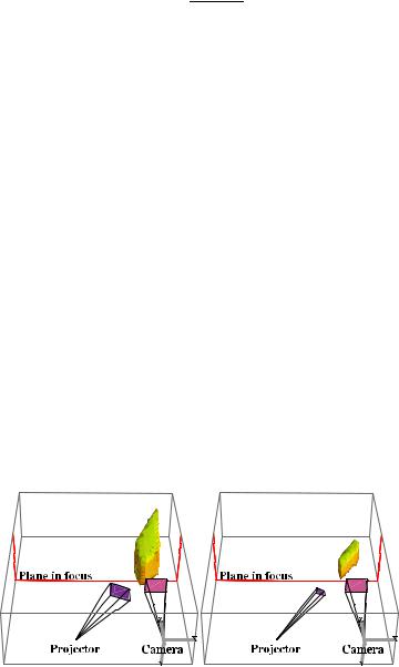
Fig. 3.9 The reconstruction volume of two systems where only the focal length of the projector is different (50 mm at left and 100 mm at right). The red lines define the plane in focus in the camera. Figure courtesy of NRC Canada