Материал: [2.1] 3D Imaging, Analysis and Applications-Springer-Verlag London (2012)
124 |
M.-A. Drouin and J.-A. Beraldin |
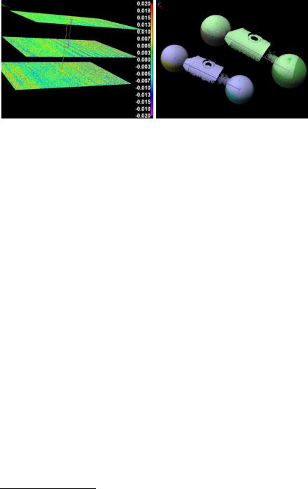
Fig. 3.13 (Left) A point-based laser scanner was used to scan the same plane at 3 different positions. The residual error in millimeters is shown using a color coding. (Right) A profile-based laser scanner was used to perform a center-to-center distance measurement between the centers of two spheres. The experiment was repeated at two different positions. Figure courtesy of NRC Canada
3.7.2 System-Level Characterization
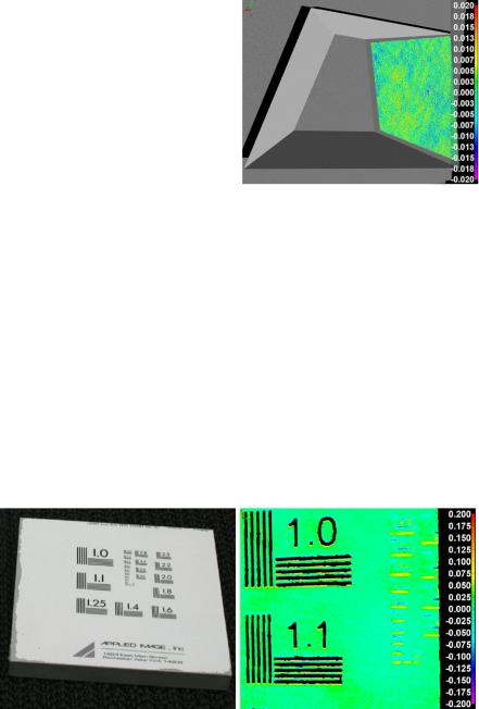
While fitting a model on a small patch of 3D points is not significantly affected by miscalibration, angle measurements are very sensitive to miscalibration. Figure 3.14 contains a 3D model of a known object produced by a fringe projection system. The nominal values of the angles between the top surface and each side are known and the difference between the values measured by fringe projection system is less than 0.03 degree. Those values were obtained by first fitting planes to the 3D points produced by the scanner and then the angles were computed. All operations were performed using the Polyworks ImInspect® software from InnovMetric.5 This experiment should be repeated using different positions and orientations of the test object. The RMSE of the plane at the right on Fig. 3.14(Top) is 10 μm.
Sphere-to-sphere measurement is part of a standard that addresses the characterization of optical measurement devices [2]. Two spheres are mounted on a bar with a known center-to-center distance. This artifact is known as a ball bar. This ball bar is placed at different predetermined positions in the reconstruction volume and the errors of center-to-center distance are used to characterize the scanner. Two scans of this object at two different positions are shown in Fig. 3.13. Again, this type of measurement is very sensitive to miscalibration.
3.7.3 Characterization of Errors Caused by Surface Properties
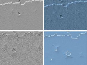
It is important to note that surface properties can significantly influence the performance of a scanner. As an example, Fig. 3.15 contains an image of a USAF resolution chart which is used to assess the lateral resolution of conventional cameras. We
5www.innovmetric.com.
3 Active 3D Imaging Systems |
125 |
Fig. 3.14 An object scanned by a fringe projection system. The nominal values of the angles between the top surface and each side are respectively 10, 20, 30 and 40 degrees. The residual error in millimeters is shown using a color coding. Figure courtesy of NRC Canada
use the chart to evaluate the impact of sharp intensity variations on the performance of scanners. Texture changes create artifacts in the surface geometry. Moreover, the light may penetrate into the surface of an object before bouncing back to the scanner and this may influence the recovered geometry [10]. Furthermore, the object surface micro-structure combined with the light source spectral distribution can greatly influence the performance of a system. As an example, an optical flat surface was scanned with the same fringe projection system using two different light sources. The first one is a tungsten-halogen source with a large wavelength range, while the second one is a red led with a narrow wavelength range. The experimentation was conducted in complete darkness and the light source intensities were adjusted such that the intensity ratios in the camera were similar for both sources. The RMSE values obtained using the two sources are 21 and 32 μm respectively (see Sect. 3.8.4).
Fig. 3.15 Intensity artifacts produced by a fringe projection system. Note that in some areas (i.e. the dark regions) the magnitude of the sinusoidal pattern was so small that the scanner did not produce any 3D points. Again, the residual error in millimeters is shown using a color coding. Figure courtesy of NRC Canada
126 |
M.-A. Drouin and J.-A. Beraldin |
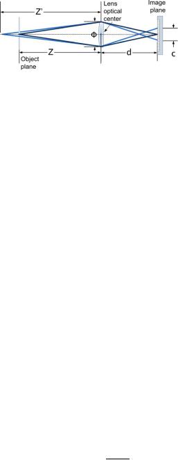
Fig. 3.16 The same surface containing defects scanned by four different scanners. (Top left) Point-based laser triangulation system. (Top right) Profile-based laser triangulation system. (Bottom left) Fringe projection system. (Bottom Right) Scanner based on conoscopic holography. Figure courtesy of [33]
3.7.4 Application-Based Characterization
We illustrate the principle behind this family of tests using a surface defect detection application. The objective of this application is to localize defects that create a variation on the surface of a product. In this type of application, the calibration of the system is not very important; however, the capability of the system to image small structural details is very important. In this test, an object which is known to contain defects is scanned and it is possible to verify the presence of those defects in the 3D data. Figure 3.16 illustrates surface defects as detected by four different systems.
3.8 Selected Advanced Topics
This section may be omitted at the first reading. It contains material that requires in-depth knowledge of the image formation process. Section 3.8.1 will present the thin lens equation. Section 3.8.2 and Sect. 3.8.3 examine the depth of field of a triangulation based 3D camera. Section 3.8.4 and Sect. 3.8.5 give some important results whose derivations would required in-depth knowledge of diffraction and Gaussian beam optics. Finally, Sect. 3.8.6 uses those results to discuss the lateral resolution of phase shift and spot scanners. Further information concerning optical issues can be found in [15, 43, 61].
3.8.1 Thin Lens Equation
Optical systems are complex and difficult to model. A very useful approximation is the thin lens equation which provides a first order approximation of a lens with
3 Active 3D Imaging Systems |
127 |
Fig. 3.17 The image of the point at distance Z from the optical center is in focus on the image plane, while the point at distance Z from the optical center is imaged as a circle of diameter c on the image plane. The lens aperture is Φ and the distance between the image plane and the optical center is d . Figure courtesy of NRC Canada
negligible thickness. Given the distance Z between an object and the optical center of the lens and the focal length f of this lens, one may compute, using the thin lens equation the distance between the optical center and the image plane needed in order to obtain a sharp image of the object. Since optical engineering falls outside the scope of this chapter, we provide the thin lens equation without derivation (see for details [61]). The thin lens equation is
1 |
1 |
1 |
|
||
|
+ |
|
= |
|
(3.45) |
Z |
d |
f |
|||
where f is the lens focal length, Z is the distance between the optical center and the object plane and d is the distance between the optical center and the image plane (i.e. the CCD or CMOS sensor).
Since d ≈ f when the distance between the camera and the object is sufficiently large, Chap. 2 and other textbooks use f (for focal length) rather than using d in their camera models (see Sect. 3.3.1).
Usually, 3D imaging systems are used for applications that require the scan of non-planar objects. Thus, Eq. (3.45) is not fulfilled for all the points on the surface of the object. As will be explained next, this induces out-of-focus blurring in some parts of the image.
3.8.2 Depth of Field
The point located at Z in Fig. 3.17, will be imaged as a circle of diameter c on the image plane. This circle is named a circle of confusion. Using simple trigonometry and the thin lens equation, the diameter of this circle can be computed as
c |
Φ |
|Z − Z| |
|
f |
(3.46) |
|
|
|
− |
||||
= |
|
Z |
|
Z |
f |
|
|
|
|
||||
where Φ is the size of the lens aperture. The proof is left as an exercise to the reader. Given a maximum diameter cmax for the circle of confusion and assuming
128 |
|
|
|
|
|
|
|
|
|
|
|
|
|
|
|
|
|
M.-A. Drouin and J.-A. Beraldin |
||||
|
|
|
|
|
|
|
|
|
|
|
|
|
|
|
|
|
|
|
|
|
|
|
|
|
|
|
|
|
|
|
|
|
|
|
|
|
|
|
|
|
|
|
|
|
|
|
|
|
|
|
|
|
|
|
|
|
|
|
|
|
|
|
|
|
|
|
|
|
|
|
|
|
|
|
|
|
|
|
|
|
|
|
|
|
|
|
|
|
|
|
|
|
|
|
|
|
|
|
|
|
|
|
|
|
|
|
|
|
|
|
|
|
|
|
|
|
|
|
|
|
|
|
|
|
|
|
|
|
|
|
|
|
|
|
|
|
|
|
|
|
|
|
|
|
|
|
|
|
|
|
|
|
|
|
|
|
|
|
|
|
|
|
|
|
|
|
|
|
|
|
|
|
|
|
|
|
|
|
|
|
|
|
|
|
|
|
|
|
|
|
|
|
|
|
|
|
|
|
|
|
|
|
|
|
|
|
|
|
|
|
|
|
|
|
|
|
|
|
|
|
|
|
|
|
|
|
|
|
|
|
|
|
|
|
|
|
|
|
|
|
|
|
|
|
|
|
|
|
|
|
|
|
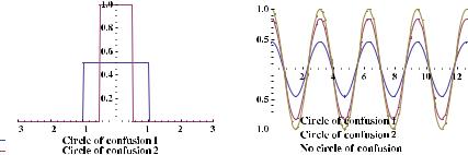
Fig. 3.18 (Left) The circle of confusion acts as a box filter. The diameter of the first circle of confusion is two units, while the diameter of the second one is one unit. (Right) Effect of blurring induced by the circles of confusion (shown left) on the magnitude of a sinusoidal pattern having a period of three units. Figure courtesy of NRC Canada
that Z > Z > f , the depth of field can be computed, using Eq. (3.46), as
Df = 2 Z − Z |
|
|
(3.47) |
|||||
where |
|
|
|
|
|
|
|
|
Z = |
|
|
Φf Z |
|
. |
(3.48) |
||
|
|
|
|
|
|
|||
Φf |
+ |
(f |
− |
Z)c |
|
|||
|
|
|
|
max |
|
|||
Thus, a large lens diameter will induce a small focusing range, even though more light is captured by the imaging system.
Figure 3.18 illustrates the impact of blurring on the magnitude of sinusoidal patterns used by a phase shift scanner. As the ratio between the circle-of-confusion diameter and spatial period of the pattern increases, the magnitude of the signal is reduced. In Eq. (3.40), it can be seen that reducing the spatial period reduces the uncertainty. However, once the optical components of the system are taken into account, one can see that reducing the spatial period, may also reduce the magnitude of the sinusoidal pattern, possibly increasing the uncertainty rather than reducing it. Furthermore, because the blurring depends on the distance of a 3D point, the magnitude of the sinusoidal pattern also depends on the distance. Thus, one should expect that the curve of standard deviation shown at Fig. 3.10, should look more like a U shape when taking into account the optically-induced blurring. It is, therefore, important to factor in the optically induced blurring and other optical related degradations when designing a system because those define the usable measurement volume, which is generally smaller than the reconstruction volume. Note than even when a system is perfectly in-focus, diffraction and aberrations induce a degradation of the image which is similar to out-of-focus blurring [61].