Материал: [2.1] 3D Imaging, Analysis and Applications-Springer-Verlag London (2012)

3 Active 3D Imaging Systems |
119 |
Sect. 3.8, when d is increased while keeping the standoff distance constant the focal length must be increased; otherwise, the image will be blurred. Note that when d is increased the field of view is also reduced. The intersection of the field of view of the camera and projector defines the reconstruction volume of a system. Figure 3.9 illustrates the reconstruction volume of two systems that differ only by the focal length of the projector (i.e. the value of d also varies). Thus, there is a trade off between the size of the reconstruction volume and the magnitude of the uncertainty.
3.6.3 Uncertainty Related to Extrinsic Parameters
Because the transformation of Eq. (3.31) from a normalized image coordinates to 3D points is non-linear, we introduce a first-order approximation using Taylor’s expansion. The solution close to xˆ2 can be approximated by
|
|
|
|
|
|
d |
|
|
|
|
||
|
|
|
|
Q(x1,y1) xˆ2 + |
x2 ≈ Q(x1,y1) xˆ2 + |
|
Q(x1,y1) xˆ2 |
|
x2 |
|
(3.42) |
|
|
|
|
|
dx2 |
|
|||||||
|
|
|
|
|
|
ˆ |
|
|
|
|
||
where |
|
|
|
|
|
|
|
|
|
|||
|
d |
|
,y1) xˆ2 |
|
|
|
|
|
|
|
||
|
|
Q(x1 |
|
|
|
|
|
|
|
|||
|
dx2 |
|
|
|
|
|
|
|
||||
|
ˆ |
|
|
|
|
|
|
x1 |
|
|
||
|
|
|
(−r33Tx + r13Tz − r31Tx x1 + r11Tzx1 − r32Tx y1 + r12Tzy1 |
) |
|
|
||||||
= |
y |
. |
(3.43) |
|||||||||
|
|
|||||||||||
|
(r13 + r11x1 − r33xˆ2 − r31x1xˆ2 + r12y1 − r32xˆ2y1)2 |
|
11 |
|
||||||||
Since a first order approximation is used, the covariance matrix associated to a 3D point can be computed similarly as ΣB in Eq. (3.35) [27, 28]. Explicitly, the covariance matrix associated with a 3D point is
|
|
x12 |
x1y1 |
x1 |
|
|
|
|
|
|
|
|
|
|
|
|
|
|
|
|
|
|
|
|
|||
Σ |
x1 |
y1 |
y12 |
y1 |
|
|
|
|
|
|
|
|
|
|
|
|
|
|
|
|
|
|
|
||||
|
= x1 |
y1 |
1 |
|
− |
|
|
+ |
|
|
|
|
− |
|
|
|
|
+ |
|
|
|
|
|
||||
|
|
|
|
− |
|
+ |
|
|
|
1 |
|
|
|
1 |
|
|
|
1 |
|
|
1 |
2 |
|||||
|
× |
|
( r33Tx |
|
r13Tz |
|
r31Tx x |
|
r11Tzx |
|
r32Tx y |
|
r12Tzy |
|
)2 |
σx2 (3.44) |
|||||||||||
|
|
|
|
(r13 |
+ |
r11x |
− |
r33x |
− |
r31x |
|
x |
+ |
r12y |
|
− |
r32x |
y |
)4 |
|
|
||||||
|
|
|
|
|
|
|
1 |
ˆ2 |
|
|
1 |
ˆ2 |
|
|
1 |
|
ˆ2 1 |
|
|
|
|
||||||
where σ 2 is computed using Eq. (3.40) and Eq. (3.41).
x2
The covariance matrix can be used to compute a confidence region which is the multi-variable equivalent to the confidence interval.4 The uncertainty over the range
4A confidence interval is an interval within which we are (1 − α)100 % confident that a point measured under the presence of Gaussian noise (of known mean and variance) will be within this interval (we use α = 0.05).
120 |
|
|
|
|
|
M.-A. Drouin and J.-A. Beraldin |
|
|
|
|
|
|
|
|
|
|
|
|
|
|
|
|
|
|
|
|
|
|
|
|
|
|
|
|
|
|
|
|
|
|
|
|
|
|
|
|
|
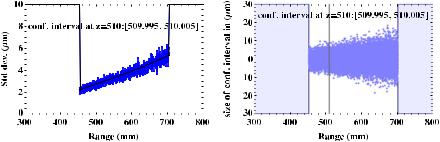
Fig. 3.10 (Left) The standard deviation obtained from the first-order approximation and the Mon- te-Carlo simulation points respectively display in black and blue. (Right) Confidence interval size computed for many range values using a first-order approximation. The Monte-Carlo simulation points are displayed at the top of the confidence interval. The reconstruction volume covers a range from 450 to 700 mm and is shown in Fig. 3.9(Left). The confidence interval for Z = 510 mm is given. Figure courtesy of NRC Canada
(i.e. Z-axis) is an important design characteristic. Figure 3.10(Left) illustrates the confidence interval for different range values for the geometric configuration at the left of Fig. 3.9. As the range increases, the size of the confidence interval also increases. This is a characteristic of triangulation systems and this explains why triangulation systems are often used for short range measurements [10]. Note that the results presented in Fig. 3.10 ignore many things such as the effect of optical components (see Sect. 3.8).
The usable measurement volume is the portion of the reconstruction volume for which the error on the position of a 3D point is expected to be smaller than a maximum permissible error. The depth of field of a scanner is the size of the interval of Z values inside this usable measurement volume. Note that because of optical limitations, such as blurring effects, the usable measurement volume can be significantly smaller than the reconstruction volume (see Sect. 3.8).
Since a first-order approximation is used when computing the uncertainty with Eq. (3.44), it is important to validate the results using Monte-Carlo simulations. Figure 3.10(Right) shows the results of one such simulation. The simulation process consisted of the following steps:
•50000 values of x2 were generated using a uniform distribution.
•Zero-mean Gaussian noise was added to each point.
•The points were triangulated using Eq. (3.31) at [x1, y1]T = [0, 0]T .
•The variance of the range values obtained previously was compared with the one computed using the first-order approximation.
3.6.4 Uncertainty as a Design Tool
For design purposes, it is useful to fix the position of a 3D point and examine how the uncertainty varies when modifying the parameters of the system. In order to do so, it
3 Active 3D Imaging Systems |
121 |
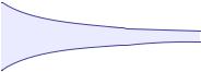
Fig. 3.11 (Left) The size of the confidence interval when varying both the vergence (i.e. the angle around the Y axis) and the baseline for the geometric configuration shown in Fig. 3.9(Left). (Right) The standard deviation for this geometric configuration. The confidence interval for a baseline value of 274 mm is given. This is the baseline value used by the geometric configuration shown in Fig. 3.9(Left). Figure courtesy of NRC Canada
is possible to modify Eq. (3.44) such that x2 is replaced by Zw . As the distance between the views is increased, the size of the uncertainty interval for the range value is reduced. Moreover, configurations with vergence produce lower uncertainty than those without, due to the preferable large angle that a back-projected ray intersects a projected plane of light. Note that the baseline and the vergence angle are usually varied together to minimize the variation of the shape and the position of the reconstruction volume. Figure 3.11 illustrates the impact of varying these extrinsic parameters of the system on the confidence interval for a fixed 3D point. As the distance between the views is increased, the amount of occlusion that occurs is also increased. An occlusion occurs when a 3D point is visible in one view but not in the other one. This can occur when a 3D point is outside the reconstruction volume of a scanner or when one part of the surface occludes another. Thus, there is a trade off between the size of the confidence interval and the amount of occlusion that may occur.
3.7 Experimental Characterization of 3D Imaging Systems
Manufacturers of 3D scanners and end-users are interested in verifying that their scanner performs within predetermined specifications. In this section, we will show scans of known objects that can be used to characterize a scanner. Objects composed of simple surfaces such as a plane or a sphere can be manufactured with great accuracy. These objects can then be scanned by the 3D imaging system and the measurements taken can be compared with nominal values. Alternatively, a coordinate measuring machine (CMM) can be used to characterize the manufactured object. This object can then be scanned by the 3D imaging system and the measurements taken can be compared with those obtained by the CMM. As a rule of thumb, the measurements acquired by the reference instrument need to be a minimum of four
122 |
M.-A. Drouin and J.-A. Beraldin |
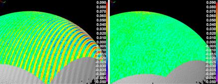
Fig. 3.12 An object scanned twice under the same conditions. A sphere was fitted to each set of 3D points. The residual error in millimeters is shown using a color coding. The artifacts visible in the left image are suspected to be the result of a human error. Figure courtesy of NRC Canada
times and preferably an order of magnitude more accurate than the measurements acquired by the 3D scanner.
We propose to examine four types of test for characterizing 3D imaging systems. Note that, the range images generated by a 3D imaging system are composed of 3D points usually arranged in a grid format. The first type of test looks at the error between 3D points that are contained in a small area of this grid. This type of test is not affected by miscalibration and makes it possible to perform a low level characterization of a scanner. The second type of test looks at the error introduced when examining the interactions between many small areas of the grid. This type of test makes it possible to perform a system level characterization and is significantly affected by miscalibration. The third family of test evaluates the impact of object surface properties on the recovered geometry. The last family of test is based on an industrial application and evaluates the fitness of a scanner to perform a given task.
In this section, we present the scans of objects obtained using different shortrange technologies. Most of the scanners used are triangulation-based and there is currently a plethora of triangulation-based scanners available on the market. Different scanners that use the same technology may have been designed for applications with different requirements; thus, a scanner that uses a given implementation may not be representative of all the scanners that use that technology. Establishing a fair comparison between systems is a challenging task that falls outside of the scope of this chapter. The results shown in this section are provided for illustration purposes.
The human operator can represent a significant source of error in the measurement chain. The user may select a 3D imaging system whose operating range or operating conditions (i.e. direct sunlight, vibration, etc.) are inadequate for a given task. Alternatively, a user can misuse a system that is well-adapted to a given task. Usually, this is a result of lack of experience, training and understanding of the performance limitations of the instrument. As an example, in Fig. 3.12, a sphere was scanned twice by the same fringe projection system under the same environmental conditions. The scan shown on the left of the figure contains significant artifacts, while the other does not. One plausible explanation for those artifacts is that the
3 Active 3D Imaging Systems |
123 |
selected projector intensity used while imaging the phase-shift patterns induces saturation for some camera pixels. Another plausible explanation is that the scanned object was inside the reconstruction volume of the scanner, but outside the usable measurement volume. Moreover, user fatigue and visual acuity for spotting details to be measured also influence the measurement chain.
3.7.1 Low-Level Characterization
Figure 3.13 shows multiple scans of a planar surface at different positions in the reconstruction volume. This type of experiment is part of a standard that addresses the characterization of the flatness measurement error of optical measurement devices [2]. When the area used to fit a plane is small with respect to the reconstruction volume, miscalibration has a very limited impact. A point-based laser triangulation scanner was used to illustrate this type of experiment. As expected from the results of the previous section, the Root Mean Square Error (RMSE) for each plane fit increases as the distance from the scanner increases (see Fig. 3.10). The RMSE values are 6.0, 7.0 and 7.5 μm. However, it is not the error value which is important but the distribution of the error which can be seen in Fig. 3.13 using a color coding. This type of experiments makes it possible to identify systematic errors that are independent of the calibration. Because of this, lens, geometric configuration and other components of the system can be changed and the system can be retested quickly. Usually, the error analysis is performed using the raw output of the scanner and not the 3D points. This makes it possible to decorrelate the different error sources and thereby simplify the identification of the error sources. As an example, for a phase-shift triangulation system, the fitting of a primitive is not performed using the [Xw , Yw , Zw ]T points obtained from the point triangulation procedure described in Sect. 3.4.3, but using the [x1, y1, x2]T directly. Moreover, in order to take into account the distortion of the lens, the rotation of the mirrors and other non-linear distortions, the raw data from the scanner is fitted to a NURBS surface rather than a plane.
We now examine an experimental protocol for measuring the error of the subpixel fringe localization of a Gray code fringe projection system [53]. It is assumed that no error in the decoding of Gray code occurs and the only error is in the subpixel localization of the fringe frontiers. Under projective geometry, the image in the camera of a projector fringe that is projected on a planar surface should remain a line. In a noise-free environment, and assuming that the line in the projector image is vertical with respect to the camera, each row y1 of the camera should provide an equation of the form [x1, y1, 1][1, a, b]T = 0 where x1 is the measured frontier and a and b are the unknown parameters defining the line. Because our camera contains more than two rows and the images are noisy, it is possible to use linear regression to estimate a and b. Once the parameters a, b of the line have been estimated, it is possible to compute the variance of the error on x1. Since the optical components introduce distortion, a projected line may no longer be a line in the camera and polynomials can be fitted rather than straight lines.