Материал: [2.1] 3D Imaging, Analysis and Applications-Springer-Verlag London (2012)

tion representation that approximates the original data. We have already seen some representations that lead to space efficient storage of 3D data. For example, subdivision surfaces require only the storage of a low resolution base mesh and subdivision rule, while the octree representation uses adaptive resolution depending on the complexity of the volume. Compression of 3D data in general [1, 49] is a more challenging problem than is solved by the relatively mature technologies available for compression of audio, image and video data. Techniques for 3D data compression can be categorized into three classes of approach:

Mesh-based methods. These methods involve traversal of a polygonal mesh and encoding of the mesh structure in a manner that can be compressed. An example of such an approach is topological surgery [69]. This method proceeds by quantizing vertex positions within the desired accuracy. A vertex spanning tree is then used to predict the position of each vertex from 2, 3 or 4 of its ancestors in the tree. Finally, the correction vectors required to recover the original positions are entropy encoded. Another popular approach is based on a spectral analysis of the mesh Laplacian [27]. An eigendecomposition of the Laplacian matrix (see Sect. 4.5.2) yields an orthonormal set of basis vectors onto which the geometry signals (vectors of x, y and z components) can be projected. By discarding high frequency components of the decomposition (i.e. those eigenvectors with small eigenvalues), the mesh can be compressed such that only high frequency detail is lost.

Progressive and hierarchical methods. We have already seen subdivision surfaces that fall into this category. Another important approach is the compressed progressive mesh [24]. In the original progressive mesh, a mesh is encoded as a form of reverse simplification. The opposite of an edge collapse operation is a vertex split, in which a vertex is divided into two and additional edges and faces are added to the mesh. A progressive mesh represents a high resolution mesh as a series of vertex split operations starting from a base mesh. Although this allows progressive transmission of increasingly detailed mesh data, there is a storage overhead, which means space requirements increase. Pajarola and Rossignac [47] showed how this representation can be compressed.

Imaged-based methods. A 3D surface may be represented in image space. This can either be native to the representation (in the case of a range image or bump map) or via a process known as surface parameterization or surface flattening [59]. Once represented as an image, any existing image compression algorithm may be applied to the data. However, it is important to note that the objectives of lossy image compression may not yield correspondingly high quality results in the surface domain since the redundancies in the two data sources may not be the same. One example of an image-based approach is geometry images [20]. Geometry is captured as a 2D array of quantized points. To transform a mesh to this representation, an arbitrary mesh is cut along a network of edge paths and the resulting single chart is parameterized onto a square. Face connectivity is implicit in the representation and bump maps or texture can be stored in the same parameterization. Compressing the resulting data using an image wavelet-encoder allows dramatic reductions in storage requirements without severely affecting the resulting geometry.

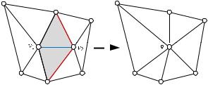
Fig. 4.19 An edge collapse operation

As suggested above, an alternative to using compression to store a high resolution mesh in less space is to derive a lower resolution mesh which approximates the original. This is known as mesh simplification and is described in the following section.

4.6.1 Mesh Simplification

Mesh simplification or mesh decimation is the process of iteratively removing vertices, edges and faces from a mesh to reduce its complexity and storage requirements. As well as reducing storage requirements by removing redundant structures, simplified meshes can also be processed or rendered more efficiently. Most mesh simplification algorithms proceed using iterative edge collapse.

4.6.1.1 Edge Collapse

A pair contraction (v1, v2) → v¯ , transforms a pair of vertices v1 and v2 to a new position v¯ , connects all their incident edges to v1 and deletes the vertex v2. Any edges or faces which became degenerate after the contraction are removed. An example is shown in Fig. 4.19.

Starting with the original high resolution mesh M N = (KN , S), a sequence of pair contractions is applied until the simplification goals are satisfied (for example, the target number of vertices is reached). Each contraction corresponds to a local incremental modification of the complex KN and shape vectors S. The algorithm generates a sequence of meshes M N , M N −1, M N −2, . . . with decreasing resolution.

In general, only edge pairs are considered valid for contraction, i.e. where

K , describing the mesh topology is modified. Degenerate faces (those that no longer have 3 distinct vertices) and duplicate edges are removed as well as the collapsed edge and redundant vertex j :

The shape vector of each individual mesh is also modified as the result of an edge collapse. The vertex vj is deleted and vi is moved to v¯ ij .

4.6.1.2 Quadric Error Metric

Edge collapse algorithms operate by selecting the next edge for collapse as the one whose deletion will result in the least increase in error. The choice of error measure determines the nature of the simplification. For example, it may seek to preserve volume or surface orientation. The most successful and widely used error measure is based on the Quadric Error Metric (QEM), as proposed by Garland and Heckbert [18] in their QSlim algorithm.

Each vertex is a solution of a set of triangles (planes), which meet at that vertex. Hence we can define the error of the vertex with respect to this set as the sum of squared distances to each triangle. Given a triangular plane p defined by the equation ax + by + cz + d = 0, where n = [a, b, c] is the plane normal and d is a scalar constant. A fundamental quadric is defined as

where A is a 3 × 3 matrix, b is a 3-vector and c is a scalar. The quadric Q assigns a value Q(v) to every point in space v by the second order equation

Note that the level surface Q(v) = ε, which is a set of all points whose error with respect to Q is ε, is a quadratic surface. Also the value of this quadratic Q(v) is precisely the squared distance of v to a given plane. The addition of quadrics can be naturally defined component-wise: Q1(v) + Q2(v) = (Q1 + Q2)(v) where (Q1 + Q2) = (A1 + A2, b1 + b2, c1 + c2). Thus, given a set of fundamental quadrics, determined by a set of planes, the quadric error at each vertex vi is completely determined by

p

where Qi = p Qp is the sum of the fundamental quadrics of all the planes incident on a vertex vi . Using this additive rule, for an edge collapse (vi , vj ) → v¯ ij , we can associate a quadric Qi+j which approximates the error at v¯ ij , where Qi+j = Qi + Qj . This simple additive rule is one of the reasons for the efficiency of this approach.

When considering the contraction of an edge (vi , vj ), we need to determine the target position v¯ ij . We select the optimum position (v¯ ) as the one that minimizes Eq. (4.33). Since Eq. (4.33) is a quadratic, finding its minimum is a linear problem.