Материал: [2.1] 3D Imaging, Analysis and Applications-Springer-Verlag London (2012)
174 |
W.A.P. Smith |
Finally, after removal of t vertices the next edge to be collapsed is chosen as the one with minimal quadric error:
i , j |
|
= |
arg min Qi |
j (vij ). |
(4.37) |
|
|
{i,j }KN −t |
+ ¯ |
|
Note that the algorithm is implemented efficiently by placing edges onto a priority queue. Priority is determined by the QEM for each edge. After each edge collapse, the QEM scores of edges sharing vertices with either end of the collapsed edge are updated (using the simple additive rule given above). Since an edge collapse is constant time complexity, the whole simplification is O(n log n), where the log n term corresponds to removing an edge from the queue. There are some additional technical considerations such as the preservation of an object boundary which are described in detail in the thesis of Garland [17].
4.6.2 QEM Simplification Summary
The QEM simplification algorithm is summarized as follows:
1.Compute quadrics for all triangles in the mesh (Eq. (4.32)).
2.Compute errors associated with all edges {i, j }: Qi+j (v¯ ij ) and place edge errors on a priority queue.
3.Delete edge with minimal error from priority queue, contract edge in mesh structure (removing redundant vertices and faces) and update QEM scores for adjacent edges.
4.If simplification goals are not met, go to step 3.
4.6.3 Surface Simplification Results
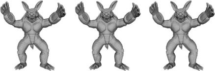
In Fig. 4.20, we show results of applying the QEM simplification algorithm to a mesh containing 172,974 vertices. The original mesh is shown on the left. The middle image shows the surface after edges have been collapsed until the number of vertices has been reduced by 80 % (to 34,595 vertices). Notice that there is almost no visual degradation of the rendering despite the large decrease in resolution. On the right, the original mesh has been simplified until the number of vertices has been reduced by 90 % (17,296 vertices remain).
4.7 Visualization
To enable humans to explore, edit and process 3D data, we require a means of visualization. The visualization of data in general is a broad and important topic
4 Representing, Storing and Visualizing 3D Data |
175 |
Fig. 4.20 Simplification results using the Quadric Error Metric. From left to right: original mesh (172,974 vertices), simplified by 80 % (34,595 vertices) and simplified by 90 % (17,296 vertices)
[29, 54] with applications in statistics and applications to scientific and medical datasets. Visualizing 3D data in particular has attracted considerable research attention, specifically where the aim is to create realistic renderings. This has been the target of computer graphics for many decades [51]. However, visualization in general encompasses a broader set of aims beyond only simulating the physics of real world image formation. For example, we may wish to navigate massive and complex datasets [71] where only a small fraction can be observed at any one time. Alternatively, our dataset may be volumetric and acquired in slices [37]. Such data can either be viewed as 2D images, formed by sampling over a plane that intersects the dataset, or rendered as 3D surfaces by applying surface fitting techniques to the raw data.
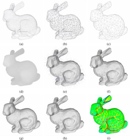
Many free tools exist for the visualization of data. In the domain of mesh data, these include MeshLab and Graphite, while for volumetric data include MicroView. In Fig. 4.21 we demonstrate some of the most common means of visualizing 3D mesh data. We begin by plotting vertices as 2D points, i.e. a point cloud. Although difficult to interpret, such visualizations can be used with raw data and give an overview of sampling density. In (b) and (c) we draw only edges, in the latter case only drawing edges which are not occluded by other faces. This gives an impression of a solid model and is easier to interpret than the raw wireframe. In (d) we show the object projected to a 2D depth map where darker indicates further away. Note that the depth data appears smooth and it is difficult to visualize small surface features when rendered in this way. In (e) we plot the vertex normals at each vertex as a blue line. Note that we use a simplified version of the surface here in order to be able to draw all of the vertex normals. In (f) we plot the principal curvature directions for the same simplified mesh as blue and red vectors. In (g) we show a smooth-shaded rendering of the original high resolution data. By varying material properties and illumination, this is the classical rendering approach used in computer graphics. In (h) we show a flat shaded rendering of the low resolution version of the mesh. In this case, triangles are shaded with a constant color which destroys the effect of a smooth surface. However, this view can be useful for inspecting the geometry of the surface without the deceptive effect of interpolation shading. Finally, in (i) we show an example of coloring the surface according to the output of a function, in
176 |
W.A.P. Smith |
Fig. 4.21 Visualization examples for mesh data: (a) point cloud, (b) wireframe, (c) wireframe with hidden surfaces removed, (d) depth map (darker indicates further away), (e) vertex normals drawn in blue, (f) principal curvature directions drawn in red and blue, (g) smooth shaded, (h) flat shaded, (i) surface color heat mapped to represent function value (in this case mean curvature)
this case mean curvature. This visualization can be useful for many surface analysis tasks. Note that the extreme red and blue values follow the lines of high curvature.
4.8 Research Challenges
Although the representation, storage and visualization of 3D data has been considered for many decades, there are still some major challenges to be faced. On the one hand, the size of 3D datasets is continuing to grow as sensing technology improves
4 Representing, Storing and Visualizing 3D Data |
177 |
(e.g. the resolution of medical imaging devices) and we begin to process large sequences of dynamic data (acquired through 4D capture) or databases of meshes. Large databases arise in applications such as 3D face recognition where fine surface detail is required to distinguish faces, yet many millions of subjects may be enrolled in the database. Not only must the database be stored efficiently but it must be possible to perform queries in real-time to be of use in real-world applications. The progressive mesh representations described above allow progressive transmission of 3D data, but this must be extended to dynamic data. Moreover, the transformation of a mesh into a progressive mesh is expensive and may not be viable for huge datasets. The growing trend to outsource storage and processing of data to “the cloud” necessitates 3D representations that can be stored, interacted with and edited in a distributed manner.
However, on the other hand, there is a growing wish to be able to access such data in a resource limited environment. For example, over bandwidth-limited network connections or on mobile devices with limited computational power. The advances in rendering technology exhibited in computer generated movie sequences will begin to find its way into consumer products such as game consoles and mobile devices. These platforms are highly resource limited in terms of both processing power and storage. Hence, the efficiency of the data structures used to store and process 3D data will be of critical importance in determining performance.
Statistical representations of 3D surfaces (such as the 3D morphable model [6]) have proven extremely useful in vision applications, where their compactness and robustness allow them to constrain vision problems in an efficient way. However, their application is limited because of model dominance whereby low frequency, global modes of variation dominate appearance. Extensions to such statistical representations that can capture high frequency local detail while retaining the compact storage requirements are a significant future challenge. A related challenge is how such models can be learnt from a sparse set of samples within a very high dimensional space, so that the model’s generalization capabilities can be improved.
4.9 Concluding Remarks
Representations of 3D data provide the interface between acquisition or sensing of 3D data and ultimately processing the data in a way that enables the development of useful applications. Anyone involved in 3D imaging and processing must be aware of the native representations used by sensing devices and the various advantages and limitations of higher level surface and volume based representations. In many cases, data in a raw representation must be preprocessed before conversion to the desired higher level format, for example through surface fitting, smoothing or resampling. Subsequently, in choosing the most suitable representation for a particular application, it must be established what operations need to be performed on the data and what requirements exist in terms of computational and storage efficiency. Whether involved with the low level design of 3D sensors or interpreting and processing high
178 |
W.A.P. Smith |
level 3D data, understanding these issues is important. Finally, as sensors and applications continue to develop, the need for new representations and methods for compression and visualization mean this remains an active research area.
4.10 Further Reading
An introductory level text covering mathematics related to geometry processing is by Vince [72]. 3D representations in general are covered in some detail in the computer graphics textbooks of Watt [73] and Foley et al. [15]. A number of textbooks focus in more detail on specific representations. For example, meshes, geometry processing algorithms including error removal, mesh creation, smoothing, conversion and morphing are covered in detail in the textbook of Botsch et al. [10]. NURBS are described in detail in the textbook of Piegl and Tiller [53], subdivision surfaces are covered by Peters and Reif [50], implicit curves and surfaces are examined by Gomes et al. [19] and the textbook of Suetens [66] deals with volumetric representations in the context of medical imaging. A popular textbook describing techniques for visualization is by Post et al. [54].
4.11 Questions
1.Compare and contrast K -d point cloud structuring and octree structuring. When might one method be preferable over the other?
2.For each of the following methods and devices for 3D acquisition, explain what is the most suitable raw data representation. Justify your answer. You may need to research how each method operates.
•Time-of-flight camera.
•Multi-view stereo.
•Shape from shading.
•Structured light.
•MRI scanner (consider structural, functional and diffusion tensor modalities).
3.For a 3D imaging application of your choice, list the operations that would need to be applied to the data and use this to guide selection of an appropriate 3D representation. Explain any difficulties that may arise in converting to this representation from the raw data acquired in your chosen application.
4.What considerations are relevant when selecting a data structure for 3D meshes?
5.Describe an application in which lossy compression of 3D data is acceptable and an application in which only lossless compression is acceptable.
6.Explain three situations in which 3D data needs to be visualized. Each situation should employ a different visualization of the data.