Материал: [2.1] 3D Imaging, Analysis and Applications-Springer-Verlag London (2012)
5 Feature-Based Methods in 3D Shape Analysis |
219 |
73.Shilane, P., Funkhauser, T.: Selecting distinctive 3D shape descriptors for similarity retrieval. In: Proc. Shape Modelling and Applications (2006)
74.Sipiran, I., Bustos, B.: A robust 3D interest points detector based on Harris operator. In: Proc. 3DOR, pp. 7–14. Eurographics (2010)
75.Sivic, J., Zisserman, A.: Video Google: A text retrieval approach to object matching in videos. In: Proc. CVPR (2003)
76.Skraba, P., Ovsjanikov, M., Chazal, F., Guibas, L.: Persistence-based segmentation of deformable shapes. In: Proc. NORDIA, pp. 45–52 (2010)
77.Sochen, N., Kimmel, R., Malladi, R.: A general framework for low level vision. IEEE Trans. Image Process. 7(3), 310–318 (1998)
78.Starck, J., Hilton, A.: Correspondence labelling for widetimeframe free-form surface matching. In: Proc. ICCV (2007)
79.Strecha, C., Bronstein, A.M., Bronstein, M.M., Fua, P.: LDAHash: improved matching with smaller descriptors. Technical Report, EPFL (2010)
80.Sumner, R.W., Popovic,´ J.: Deformation transfer for triangle meshes. In: Proc. Conf. Computer Graphics and Interactive Techniques, pp. 399–405 (2004)
81.Sun, J., Ovsjanikov, M., Guibas, L.: A concise and provably informative multi-scale signature based on heat diffusion. Comput. Graph. Forum 28(5), 1383–1392 (2009)
82.Thorstensen, N., Keriven, R.: Non-rigid shape matching using geometry and photometry. In: Proc. CVPR (2009)
83.Toldo, R., Castellani, U., Fusiello, A.: Visual vocabulary signature for 3D object retrieval and partial matching. In: Proc. 3DOR (2009)
84.Torresani, L., Kolmogorov, V., Rother, C.: Feature correspondence via graph matching: models and global optimization. In: Proc. ECCV, pp. 596–609 (2008)
85.Wang, C., Bronstein, M.M., Bronstein, A.M., Paragios, N.: Discrete minimum distortion correspondence problems for non-rigid shape matching. In: Proc. Conf. on Scale Space and Variational Methods in Computer Vision (SSVM) (2011)
86.Wardetzky, M., Mathur, S., Kälberer, F., Grinspun, E.: Discrete Laplace operators: no free lunch. In: Conf. Computer Graphics and Interactive Techniques (2008)
87.Zaharescu, A., Boyer, E., Varanasi, K., Horaud, R.: Surface feature detection and description with applications to mesh matching. In: Proc. CVPR (2009)

Chapter 6
3D Shape Registration
Umberto Castellani and Adrien Bartoli
Abstract Registration is the problem of bringing together two or more 3D shapes, either of the same object or of two different but similar objects. This chapter first introduces the classical Iterative Closest Point (ICP) algorithm, which represents the gold standard registration method. Current limitations of ICP are addressed and the most popular variants are described to improve the basic implementation in several ways. Challenging registration scenarios are analyzed and a taxonomy of recent and promising alternative registration techniques is introduced. Three case studies are then described with an increasing level of problem difficulty. The first case study describes a simple but effective technique to detect outliers. The second case study uses the Levenberg-Marquardt optimization procedure to solve standard pairwise registration. The third case study focuses on the challenging problem of deformable object registration. Finally, open issues and directions for future work are discussed and conclusions are drawn.
6.1 Introduction
Registration is a critical issue for various problems in computer vision and computer graphics. The overall aim is to find the best alignment between two objects or between several instances of the same object, in order to bring the shape data into the same reference system. The main high level problems that use registration techniques are:
1.Model reconstruction. The goal in model reconstruction is to create a complete object model from partial 3D views obtained by a 3D scanner. Indeed, it is rare that a single 3D view captures the whole object structure, mainly due to self occlusions. Registration allows one to obtain the alignment between the partial
U. Castellani ( ) |
|
|
|
University of Verona, Verona, Italy |
|
e-mail: Umberto.Castellani@univr.it |
|
A. Bartoli |
|
Université d’Auvergne, Clermont-Ferrand, France |
|
e-mail: Adrien.Bartoli@gmail.com |
|
N. Pears et al. (eds.), 3D Imaging, Analysis and Applications, |
221 |
DOI 10.1007/978-1-4471-4063-4_6, © Springer-Verlag London 2012 |
|
222 |
U. Castellani and A. Bartoli |
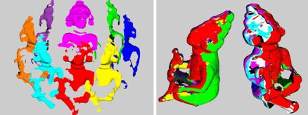
Fig. 6.1 Example of model reconstruction. Partial 3D views of the object of interest are acquired (left). After registration all the 3D views are transformed to the common reference system and merged (right). Figure generated by Alessandro Negrente, reproduced from [34]
overlapping 3D views in order to build a complete object model, also called a mosaic (see Fig. 6.1). In this context, registration is first applied between pairs of views [7, 78]. The whole model is then reconstructed using multiple view registration refinement [43, 78]. Typically, model reconstruction is employed in cultural heritage [6] to obtain 3D models of archaeological findings. It has also been applied in applications such as reverse engineering and rapid prototyping [95] and for vision in hostile environments [17, 18].
2.Model fitting. The goal in model fitting is to compute the transformation between a partial 3D view and a known CAD model of the actual object. Model fitting is used in robotics for object grasping [25, 64] and model-based object tracking [75]. Model fitting is typically used with rigid objects but has recently been extended to deformable objects [19].
3.Object recognition. The goal in object recognition is to find, amongst a database of 3D models, which one best matches an input partial 3D view. This problem is more challenging than model fitting since a decision has to be made regarding which model, if any, is the sought one. Solving the recognition problem this way is called recognition-by-fitting [92]. Several works have been done for 3D face recognition [9, 10, 83] and for 3D object retrieval [33, 90]. Registration becomes more challenging in a cluttered environment [4, 47, 56].
4.Multimodal registration. The goal in multimodal registration is to align several views of the same object taken by different types of acquisition systems. After registration, the information from different modalities can be merged for comparison purposes or for creating a multimodal object model. This problem is typical in medical imaging where it is common to register MRI and CT scans or MRI and PET scans [54, 84]. 3D medical image registration is discussed further in Chap. 11.
This chapter gives a general formulation for the registration problem. This formulation leads to computational solutions that can be used to solve the four above mentioned tasks. It encompasses most of the existing registration algorithms. For a
6 3D Shape Registration |
223 |
detailed description of registration techniques and experimental comparisons, we refer the reader to recent surveys [48, 57, 76, 78, 79]. It is worth mentioning that most of the existing computational solutions are based on the seminal Iterative Closest Point (ICP) [7] algorithm that we will describe shortly.
Chapter Outline This chapter is organized as follows. We first present the twoview registration problem and the current algorithmic solutions. We then describe some advanced registration techniques. We give a comprehensive derivation of algorithms for registration by proposing three case studies. We give an overview of open challenges with future directions and conclusions. Finally, suggestions for further reading, questions and exercises are proposed.
6.2 Registration of Two Views
Firstly we give a mathematical formulation of the two-view registration problem and then derive the basic ICP algorithm and discuss its main variants.
6.2.1 Problem Statement
Given a pair of views D and M representing two scans (partial 3D views) of the same object, registration is the problem of finding the parameters a of the transformation function T (a, D) which best aligns D to M. Typically, D and M are either simple point clouds or triangulated meshes [15]. The moving view D is called the data-view, while the fixed view M is called the model-view. The registration problem is solved by estimating the parameters a of the transformation T that satisfy:
a |
= |
a |
T (a, D), M , |
(6.1) |
|
arg min E |
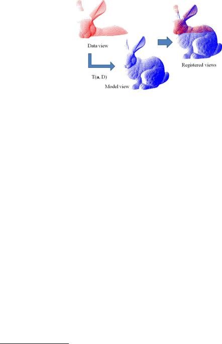
where E is called the error function and measures the registration error. Figure 6.2 illustrates the two-view registration process. The data-view and the model-view show different portions of Bunny. The transformation function T (a, D) is applied and the registered views are shown.
Most of the registration methods are based on the paradigm defined directly above and differ in the following aspects:
The transformation function. The transformation function T usually implements a rigid transformation of the 3D space. It uses a translation vector t and a rotation matrix R whose values are encoded or parametrized in the parameter vector a. The transformation function may also handle deformations; this requires a more complex formulation.
224 |
U. Castellani and A. Bartoli |
Fig. 6.2 Pairwise registration. The data-view and the model-view (left) are to be registered. The transformation function
T (a, D) allows one to move the data-view to the model-view’s coordinate frame (right) to align the two views
The error function. The error function E measures the registration error or dissimilarity between D and M after alignment. When the transformation function T is rigid, E is a measure of congruence between the two views. In general E takes the form of an L2 approximation of the Hausdorff distance, which further involves the so-called point-to-point distance [7] or the point-to-plane distance [23].
The optimization method. This is the method or algorithm used to find the minimizer a in Eq. (6.1). The gold standard is the iterative approach used in the ICP algorithm [7], which was specifically designed for the problem at hand. General purpose optimization methods such as Levenberg-Marquardt [32] have also been used for this problem.
6.2.2 The Iterative Closest Points (ICP) Algorithm
In the classical ICP algorithm [7] the overall aim is to estimate a rigid transformation with parameters a = (R, t). Both views are treated as point clouds D = {d1, . . . , dNd } and M = {m1, . . . , mNm }. The error function is chosen as:
|
|
|
|
|
|
Nd |
|
|
|
|
|
|
|
|
2, |
|
E |
ICP |
(a, D, M) |
= |
(Rd |
i + |
t) |
− |
m |
(6.2) |
|||||||
|
|
|
|
|
|
|
|
|
j |
|
||||||
|
|
|
|
= |
|
i=1 |
|
|
|
|
|
|
|
|
|
|
1 |
|
|
|
E(T (a, D), M) and where (di , mj ) are corre- |
||||||||||||
where we define EICP(a, D, M) |
|
|||||||||||||||
sponding points [78]. |
Fixing di |
D the corresponding point mj M is computed |
||||||||||||||
such that: |
|
= |
|
|
|
|
i + |
|
− |
|
|
k |
|
|
||
|
|
|
|
|
|
t) |
m |
|
|
|||||||
|
j |
|
arg min |
(Rd |
|
|
|
|
2. |
(6.3) |
||||||
k{1,...,Nm}
1Note that the pair (di , mj ) is initially a tentative correspondence, which becomes a true correspondence when convergence to a global minimum is attained.